
9 Lab: Support Vector Machines
This is a modified version of the Lab: Support Vector Machines section of chapter 9 from Introduction to Statistical Learning with Application in R (ISLR). This version differs from the ISLR lab in that it uses tidyverse techniques and methods that will allow for scalability and a more efficient data analytic pipeline.
9.1 Libraries
In this lab, we will only need two additional libraries e1071, which contains the function used to fit SVM in R, as well as the pROC library to examine the accuracy of our models.
# Fitting and examining SVM
library(e1071)
library(pROC)

# Wrangling, plotting, etc.
library(tidyverse)
9.2 Data
In this lab, the authors of ISLR create a synthetic (simulated) dataset. Here, we expand their code so that it runs within the tidyverse workflow. This involves creating a helper function:
# helper function to make svm dataset
#' @name make_svm_df
#' @param n_obs integer, number of rows in df
#' @returns data frame with n_obs rows, an outcome 'y', and
#'          and two predictors 'x1', 'x2'
make_svm_df <- function(n_obs){

  if(n_obs %% 2 == 1){
    n_obs = n_obs + 1
  }

  dat <- tibble(x1 = rnorm(n_obs),
                x2 = rnorm(n_obs),
                y = rep(c(-1, 1), each = n_obs/2)) %>%
    mutate(x1 = x1 + as.integer(y == 1),
           x2 = x2 + as.integer(y == 1),
           y = as.factor(y))

  return(dat)
}
We can then create a tibble of synthetic training and test data, and we can visualize the classification problem in the training set using ggplot().
set.seed(549331)
n_train = 1000
n_test = 500

# make svm data tibble
svm_dat <- tibble(train = make_svm_df(n_train) %>% list(),
                  test = make_svm_df(n_test) %>% list())

# visualize svm data
svm_dat %>%
  pluck("train", 1) %>%
  ggplot() +
    geom_point(aes(x1, x2, color = factor(y)))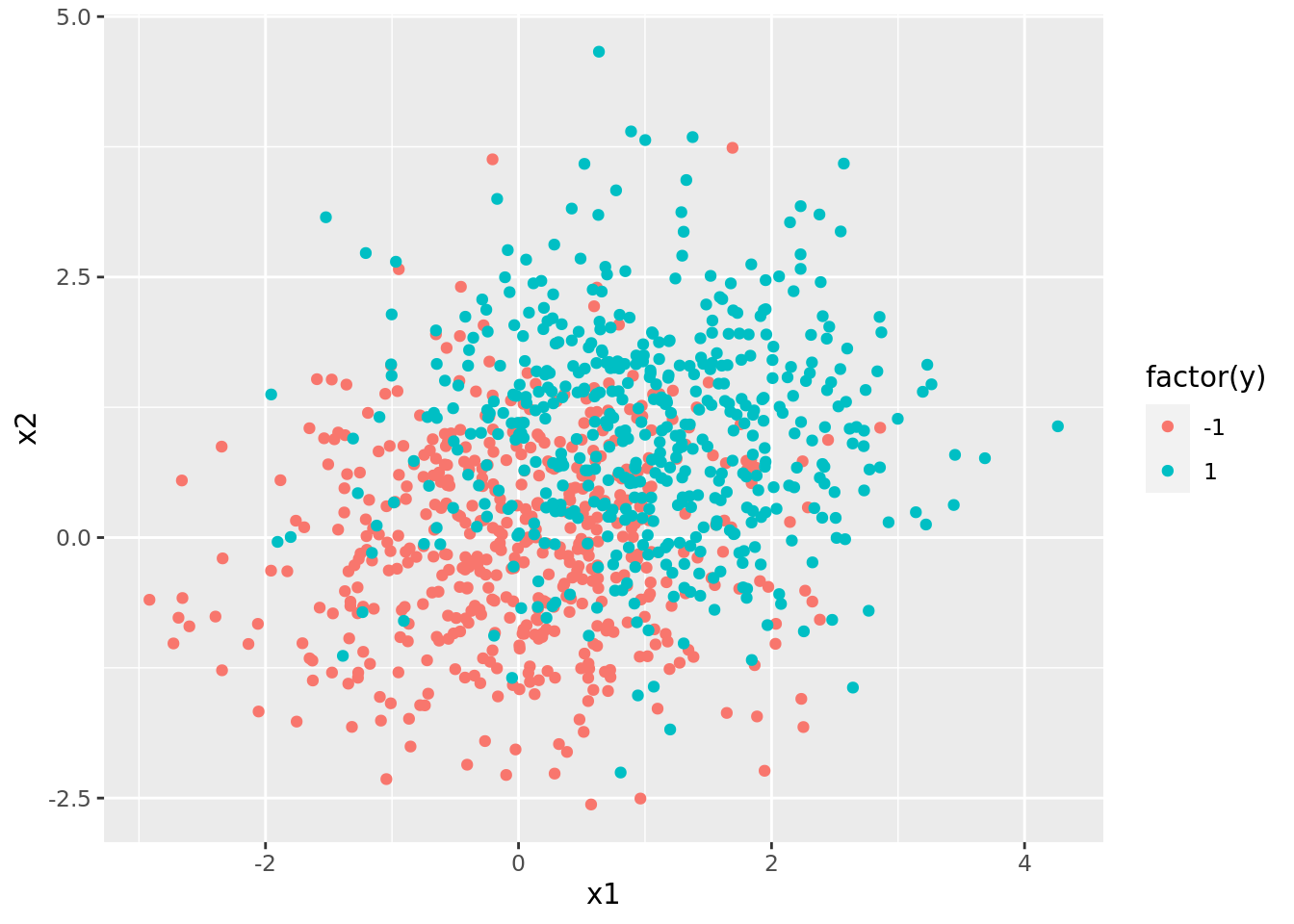
Note that there is overlap in the classes (i.e., the different colored points are all mixed together). Thus, we will not be able to make a clear hard-margin classifier, and must instead use SVM.
9.3 Fitting Linear SVM
We are now ready to fit some basic SVM models. The function that does this in R is svm(). This takes some familiar arguments, such as formula and data, but we can also specify the kernel used (kernel), as well as the soft-margin budget parameter \(C\) (cost).
Fitting a basic linear SVM looks like this:
svm_mods <- svm_dat %>%
crossing(tibble(cost = list(0.1, 1, 10))) %>%
mutate(svm_linear = map2(.x = train, .y = cost,
.f = function(x, y) svm(y ~ ., x, kernel = "linear", cost = y)), # fit svm model
svm_linear_summary = map(svm_linear, summary), # summaries of models
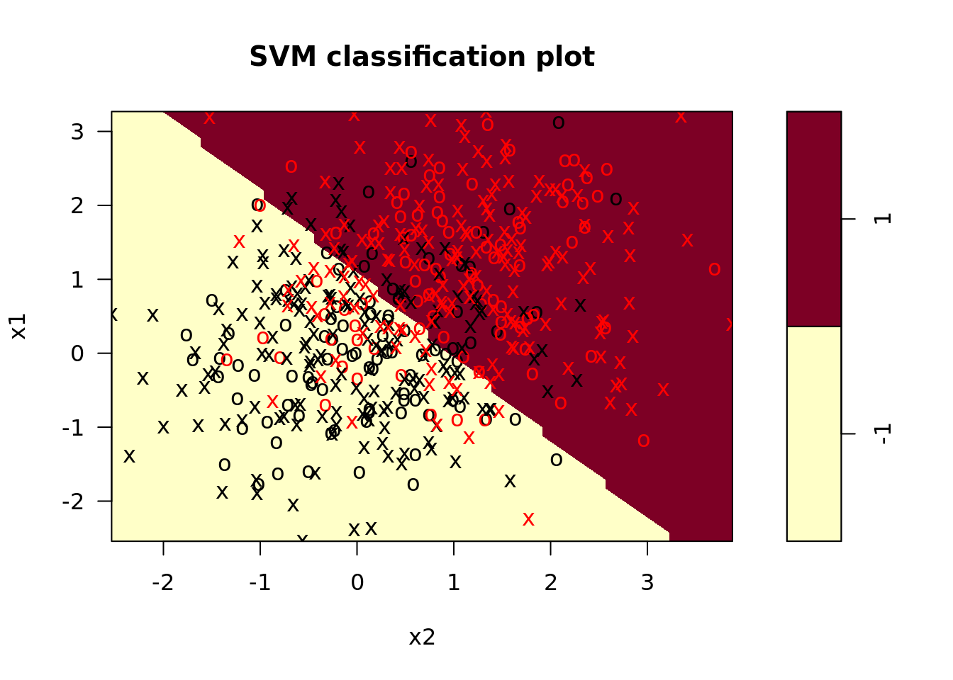
svm_linear_plot = map2(svm_linear, train, plot)) # plot svm model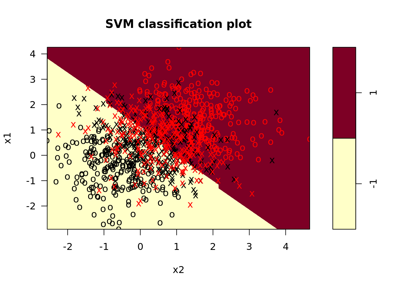

These plots look a little dated; how might you write a helper function in ggplot to make them look more modern? Try it on your own!
Recall that features should be standardized prior to fitting an SVM. Since the data we generated in the previous section is all on the same scale, this is not necessary for this lab. However, for reference, it is worth noting that there are two ways to do this in the tidyverse workflow. The first way is to pre-preprocess your data (i.e., prior to fitting a model) using, for example, the scale() function. The result is a data frame that has scaled feature values, which you then feed into the svm() function. The second way to handle this is to use the scale argument in the svm() function. Here, you can feed in unscaled data, and the svm() function will automatically scale features. You can even specify which features to scale!
While we might be tempted compare the outputs of these models, recall that cost is a tuning parameter, and thus ought to be evaluated through cross-validation or some other estimate of test error. While it is possible to use the modelr framework for cross-validation, it happens that there is a cross-validation function called tune() that can be helpful. As arguments, tune takes the function called to fit the model (here, svm), the training data, and other arguments we might want to fix. It also takes an argument called ranges which is a list of parameters you wish to tune and the values you want to try to tune them to:
svm_cv <- svm_dat %>%
  mutate(tune_svm_linear = map(.x = train,
                               .f = function(x){
                                      return(tune(svm, y ~., data = x, kernel = "linear",
                                             # let cost range over several values
                                             ranges = list(cost = c(0.01, 0.1, 1, 5, 10, 50, 100, 500)))
                                           )
                                 }))

linear_params <- svm_cv %>%
  pluck("tune_svm_linear", 1) %>%
  pluck("best.parameters")

linear_params
## cost
## 1 0.01Note that this 10-fold cross-validation approach tells us that the best value of cost is probably 0.01. To get a sense of the test error when \(C =\) 0.01 we can re-run the model and examine a confusion matrix on the test set. Here, we will use the confusionMatrix() function from the caret pacakge:
svm_linear_model <- svm_dat %>%
mutate(model_fit = map(.x = train, # fit the model
.f = function(x) svm(y ~ ., data = x, cost = linear_params$cost, kernel = "linear")),
test_pred = map2(model_fit, test, predict), # get predictions on test set
confusion_matrix = map2(.x = test, .y = test_pred, # get confusion matrix
.f = function(x, y) caret::confusionMatrix(x$y, y)),
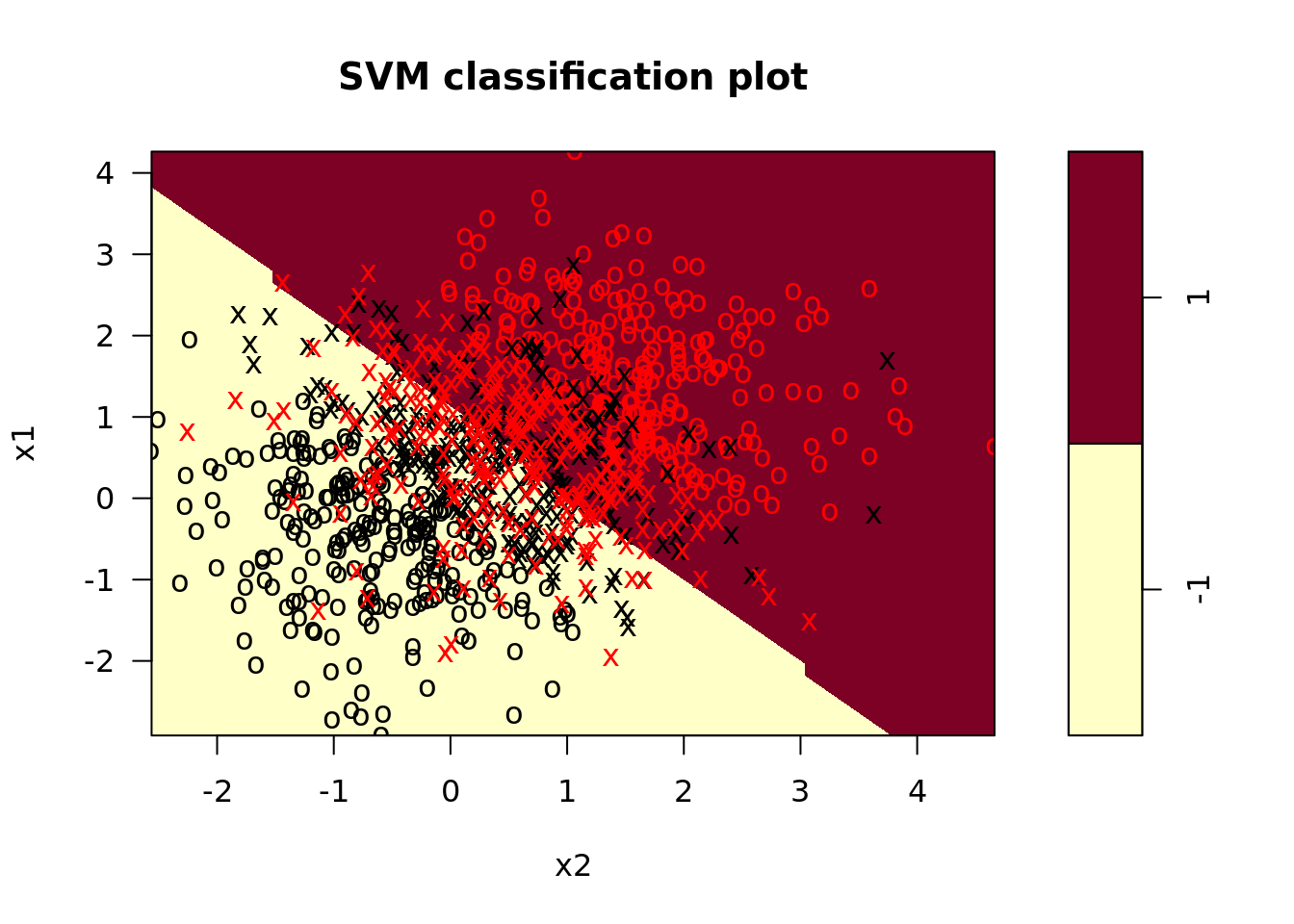
plot_train = map2(model_fit, train, plot), # plot the model on the training data
plot_test = map2(model_fit, test, plot)) # plot the model on the test data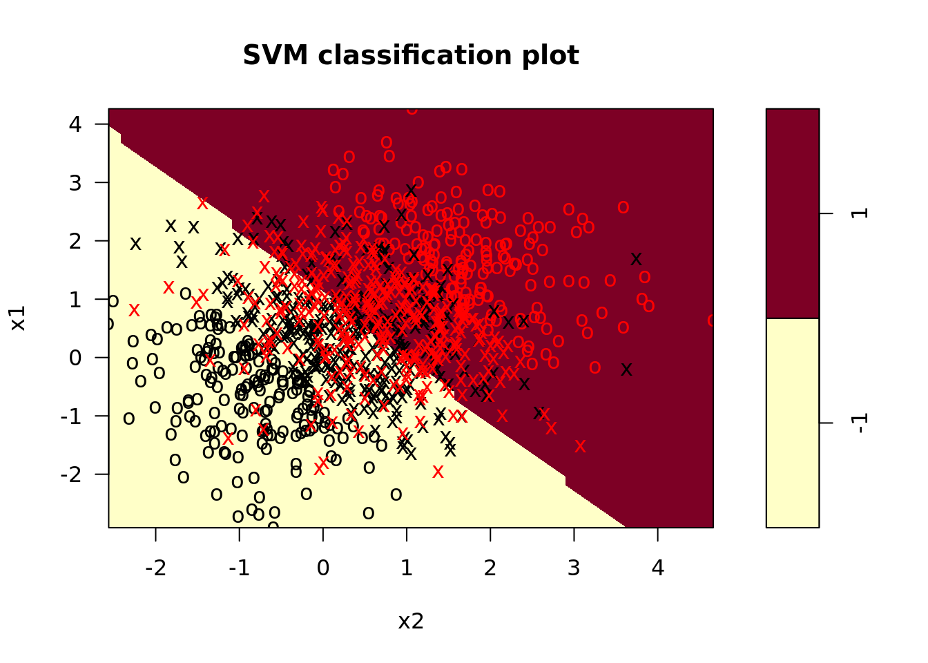
svm_linear_model %>% pluck("confusion_matrix", 1)## Confusion Matrix and Statistics
##
## Reference
## Prediction -1 1
## -1 193 57
## 1 54 196
##
## Accuracy : 0.778
## 95% CI : (0.739, 0.8137)
## No Information Rate : 0.506
## P-Value [Acc > NIR] : <2e-16
##
## Kappa : 0.556
##
## Mcnemar's Test P-Value : 0.8494
##
## Sensitivity : 0.7814
## Specificity : 0.7747
## Pos Pred Value : 0.7720
## Neg Pred Value : 0.7840
## Prevalence : 0.4940
## Detection Rate : 0.3860
## Detection Prevalence : 0.5000
## Balanced Accuracy : 0.7780
##
## 'Positive' Class : -1
## From the confusion matrix, we see that the majority of test observations are correctly classified.
9.4 SVM with Non-linear Decision Boundaries
In this section, we will fit SVM with non-linear decision boundaries. Recall that we can use basis expansion functions (or kernels) with SVM that do not dramatically increase the computational load for fitting the model. We can specify which kernel we want to use with the kernel argument in svm(). In this section, we’ll focus on using the radial kernel, which has an additional tuning parameter, \(\lambda\).
9.4.1 Data
To make it worth our while to fit a non-linear decision boundary, we need data that requires it. Thus we will need to expand our helper function from above in order to generate data with nonlinear classification rules:
# helper function to make svm dataset
#' @name make_svm_nonlinear_df
#' @param n_obs integer, number of rows in df
#' @returns data frame with n_obs rows, an outcome 'y', and
#'          and two predictors 'x1', 'x2'
make_svm_nonlinear_df <- function(n_obs){

  if(n_obs %% 2 == 1){
    n_obs = n_obs + 1
  }

  dat <- tibble(x1 = rnorm(n_obs, sd = 0.95),
                x2 = rnorm(n_obs, sd = 0.95)) %>%
    mutate(y = as.integer((pnorm(x1) + pnorm(x2) +
                             rnorm(n(), sd = 0.1) < 1) |
                                (x1^2 + x2^2 < 0.99)),
           y = as.factor(y)) # set y as a factor

  return(dat)
}
We can now use this to make a similar tibble as the previous section:
set.seed(2222222) # Glen Lerner

# make svm data tibble
svm_nl_dat <- tibble(train = make_svm_nonlinear_df(n_train) %>% list(),
                     test = make_svm_nonlinear_df(n_test) %>% list())

# visualize svm data
svm_nl_dat %>%
  pluck("train", 1) %>%
  ggplot() +
    geom_point(aes(x1, x2, color = factor(y)))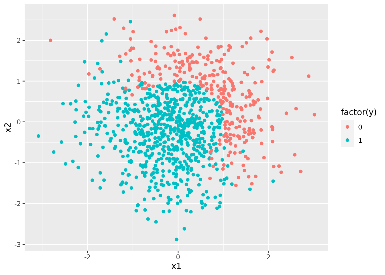
Clearly, a single straight line cannot divide these categories, so we will need to use a nonlinear kernel.
9.4.2 Polynomial Basis Expansion
With polynomial basis expansions, SVM have three tuning parameters: cost, degree, and gamma. We can cross-validate which values of these we should use in our final model. Here, we implement cross-validation with the tune() function. However, because of the computational cost, we will focus on tuning just two of these parameters: cost and degree:
set.seed(1)
svm_poly_cv <- svm_nl_dat %>%
  mutate(train_cv = map(.x = train,
                        .f = function(x) tune(svm, y ~ ., data = x, kernel = "polynomial",
                                              ranges = list(cost = c(0.1, 1, 10, 50, 100, 500),
                                                            degree = c(2, 3),
                                                            tunecontrol = tune.control(cross = 5))
                                              )
                        ))
poly_params <- svm_poly_cv %>%
  pluck("train_cv", 1)  %>%
  pluck("best.parameters")

poly_params
## cost degree tunecontrol
## 9 10 3 FALSEGiven the results above, it appears that a cost of 10 and a polynomial expasion of degree 3 are the best combination. Note however, we may want to revisit certain values or tune over a finer range of values!
Thus we can fit the model using those values:
svm_poly <- svm_nl_dat %>%
  mutate(model_fit = map(.x = train,
                         .f = function(x) svm(y ~ ., data = x, kernel = "polynomial",
                                              cost = poly_params$cost,
                                              degree = poly_params$degree,
                                              probability = TRUE)))
To study our model performance on the test set and to help visualize our SVM, we can use the following chunk:
svm_poly <- svm_poly %>%
  mutate(train_pred = map2(model_fit, train, predict, probablilty = TRUE), # training predictions for ROC later
         test_pred = map2(model_fit, test, predict, probability = TRUE), # test predcitions
         test_confusion = map2(.x = test, .y = test_pred, # test confusion matrix
                               .f = function(x, y) caret::confusionMatrix(x$y, y)),
         plot_train = map2(model_fit, train, plot), # plot training data
         plot_test = map2(model_fit, test, plot)) # plot test data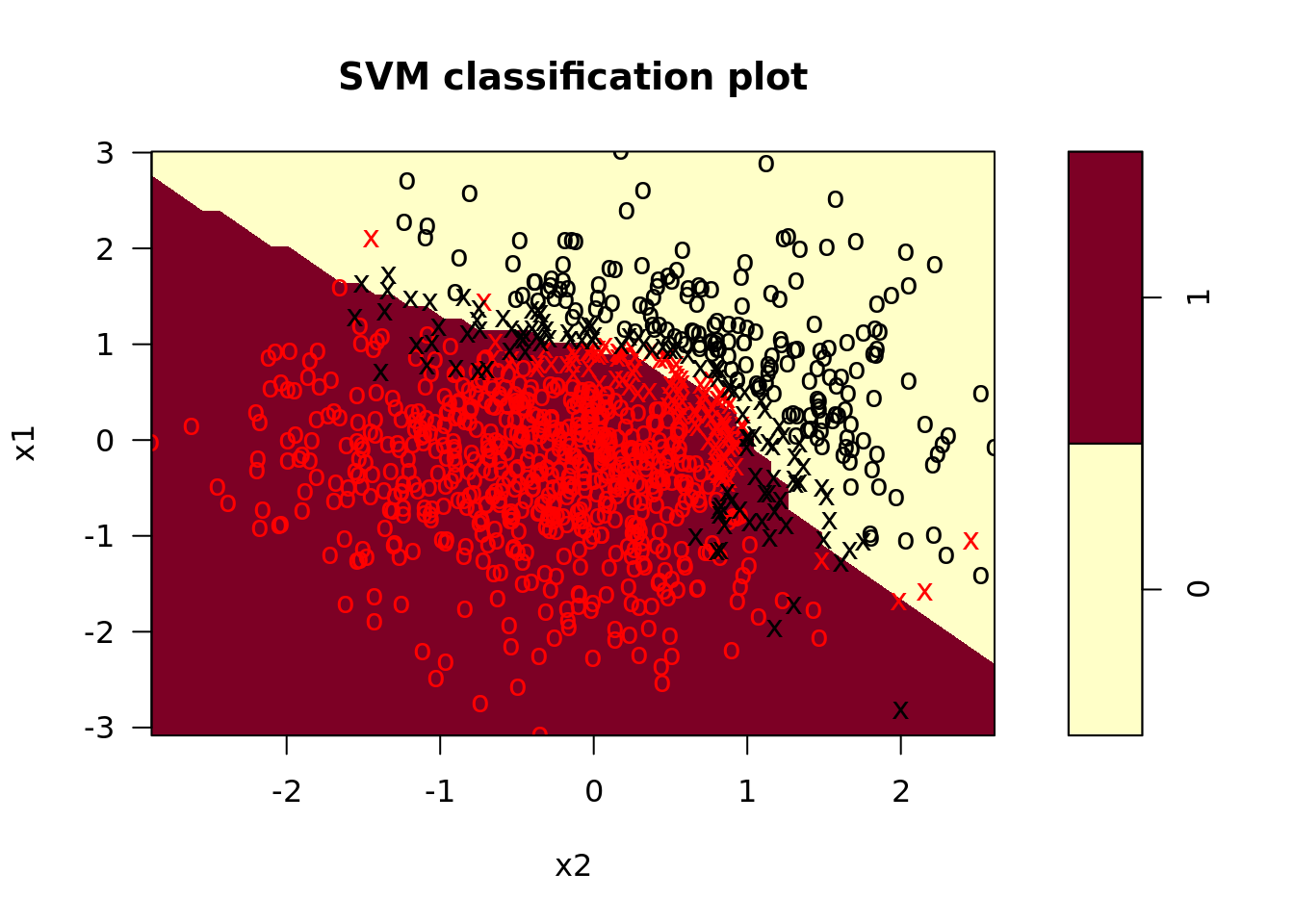
In the plots, we see that the radial kernel SVM does a decent job picking up the nonlinear decision boundary. On our test set, the performance looked like this:
svm_poly %>%
  pluck("test_confusion", 1)
## Confusion Matrix and Statistics
##
## Reference
## Prediction 0 1
## 0 116 43
## 1 1 340
##
## Accuracy : 0.912
## 95% CI : (0.8837, 0.9353)
## No Information Rate : 0.766
## P-Value [Acc > NIR] : < 2.2e-16
##
## Kappa : 0.7817
##
## Mcnemar's Test P-Value : 6.37e-10
##
## Sensitivity : 0.9915
## Specificity : 0.8877
## Pos Pred Value : 0.7296
## Neg Pred Value : 0.9971
## Prevalence : 0.2340
## Detection Rate : 0.2320
## Detection Prevalence : 0.3180
## Balanced Accuracy : 0.9396
##
## 'Positive' Class : 0
## This shows that the vast majority of test observations were correctly classified!
9.4.3 Radial Basis Expansion
Recall that with radial kernels, SVM have two tuning parameters: cost and gamma. Cross validation, implemented here with the tune() function, can help us find which values of these parameters produces the best model.
set.seed(1)
svm_nl_cv <- svm_nl_dat %>%
  mutate(train_cv = map(.x = train,
                        .f = function(x) tune(svm, y ~ ., data = x, kernel = "radial",
                                              ranges = list(cost = c(0.1, 1, 10, 50, 100, 200, 500),
                                                            gamma = seq(0.1, 10, length.out = 5))
                                              )
                        ))
radial_params <- svm_nl_cv %>%
  pluck("train_cv", 1)  %>%
  pluck("best.parameters")

radial_params
## cost gamma
## 7 500 0.1From the cross validation, it appears that a cost of 500 and a gamma of 0.1 are the best combination. Note, however, we can and should revisit the values we tuned over.
Given these values of cost and gamma, we can fit our model on the entire training set with:
svm_nl <- svm_nl_dat %>%
  mutate(model_fit = map(.x = train,
                         .f = function(x) svm(y ~ ., data = x, kernel = "radial",
                                              cost = radial_params$cost, gamma = radial_params$gamma,
                                              probability = TRUE)))
We might want to know how our model performs on the test set, and we might want to visualize the SVM:
svm_nl <- svm_nl %>%
mutate(train_pred = map2(model_fit, train, predict, probablilty = TRUE), # training predictions for ROC later
test_pred = map2(model_fit, test, predict, probability = TRUE), # test predcitions
test_confusion = map2(.x = test, .y = test_pred, # test confusion matrix
.f = function(x, y) caret::confusionMatrix(x$y, y)),
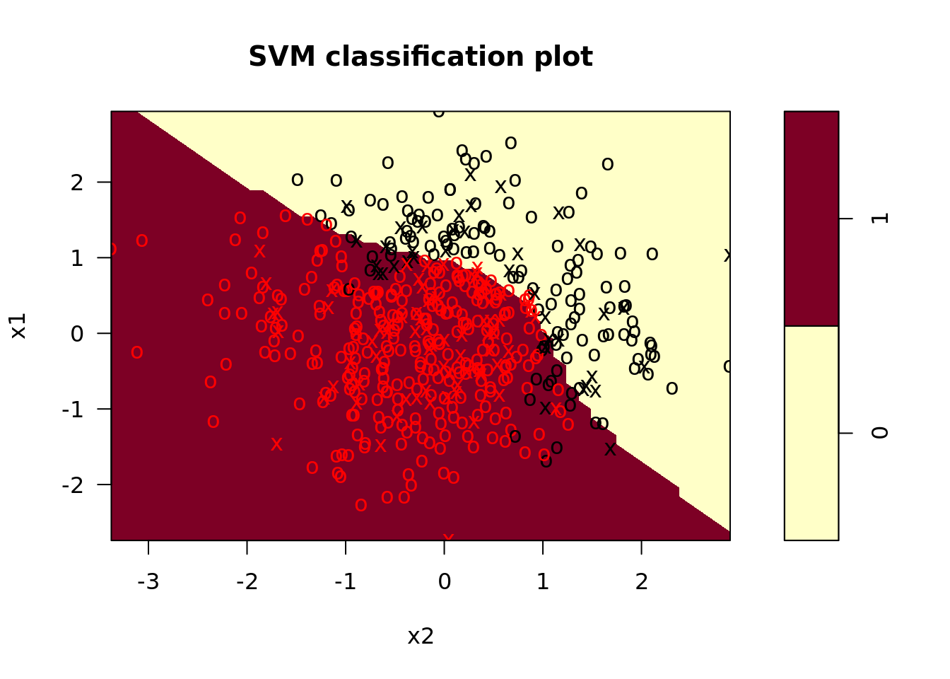
plot_train = map2(model_fit, train, plot), # plot training data
plot_test = map2(model_fit, test, plot)) # plot test data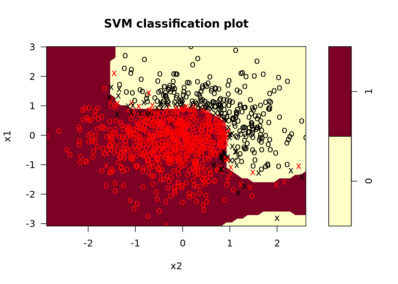
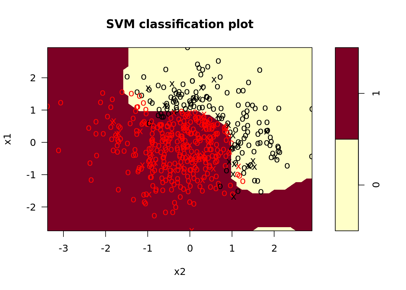
In the plots, we see that the radial kernel SVM does a decent job picking up the nonlinear decision boundary. On our test set, the performance looked like this:
svm_nl %>%
  pluck("test_confusion", 1)
## Confusion Matrix and Statistics
##
## Reference
## Prediction 0 1
## 0 141 18
## 1 8 333
##
## Accuracy : 0.948
## 95% CI : (0.9247, 0.9658)
## No Information Rate : 0.702
## P-Value [Acc > NIR] : < 2e-16
##
## Kappa : 0.8781
##
## Mcnemar's Test P-Value : 0.07756
##
## Sensitivity : 0.9463
## Specificity : 0.9487
## Pos Pred Value : 0.8868
## Neg Pred Value : 0.9765
## Prevalence : 0.2980
## Detection Rate : 0.2820
## Detection Prevalence : 0.3180
## Balanced Accuracy : 0.9475
##
## 'Positive' Class : 0
## How does this compare with the polynomial model above?
9.4.4 ROC Curves
We can generate ROC curves to get a better sene of model performance using the pROC library. This library uses functions to create ROC-type data, called roc(), and it has a funciton to plot this data in ggplot2 called ggroc(). When using these operations, it helps to have some helper functions to extract classification probabilities, as well as generate ROC-type data:
get_probs <- function(pred){
  attributes(pred)$probabilities %>%
    as_tibble() %>%
    rename(X1 = `1`) %>%
    select(X1) %>%
    as_vector() %>%
    return()
}

roc_svm <- function(data, pred){
  pROC::roc(data$y, pred)
}
Now we can create ROC curves for the test data:
svm_roc <- svm_nl %>%
  mutate(test_pred_prob = map(test_pred, get_probs),
         test_roc = map2(test, test_pred_prob, roc_svm),
         test_roc_plot = map(test_roc, ggroc))
## Setting levels: control = 0, case = 1## Setting direction: controls < casessvm_roc %>%
pluck("test_roc_plot", 1)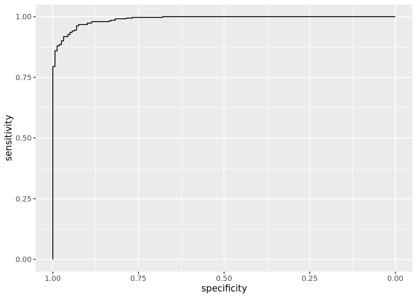
How might you go about doing the same thing for the training data?