
7 Lab: Non-linear Modeling
This is a heavily modified version of the Lab: Non-linear Modeling section of chapter 7 from Introduction to Statistical Learning with Application in R. This version uses tidyverse techniques and methods that will allow for scalability and a more efficient data analytic pipeline. We also utilize a Pokémon dataset1. We have processed the dataset a little for use in this lab. Students can find the pokemon_modified.csv on the course’s Canvas page.
We will need the packages loaded below.
# Load packages
library(tidyverse)
library(modelr)
library(naniar)

# new package
library(rsample)
7.1 Data Setup
A codebook for the original dataset can be found at https://www.kaggle.com/rounakbanik/pokemon. Maybe take a moment and inspect the codebook.
Our goal will be to demonstrate the use of non-linear techniques to predict capture_rate with base_total.
The lower the capture_rate a Pokémon has, the more difficult it is to capture. The variable base_total is actually the sum of six base attributes: hp, sp_attack, sp_defense, speed, defense, and attack.
# read in data
pokemon_dat <- read_csv("data/pokemon_modified.csv") %>%
  mutate(
    generation = factor(generation),
    is_legendary = factor(is_legendary)
  )

# check missingness
miss_var_summary(pokemon_dat) %>%
  arrange(desc(n_miss))
FALSE # A tibble: 20 x 3
FALSE variable n_miss pct_miss
FALSE <chr> <int> <dbl>
FALSE 1 percentage_male 98 12.2
FALSE 2 height_m 20 2.50
FALSE 3 weight_kg 20 2.50
FALSE 4 capture_rate 1 0.125
FALSE 5 attack 0 0
FALSE 6 base_egg_steps 0 0
FALSE 7 base_happiness 0 0
FALSE 8 base_total 0 0
FALSE 9 defense 0 0
FALSE 10 experience_growth 0 0
FALSE 11 hp 0 0
FALSE 12 japanese_name 0 0
FALSE 13 name 0 0
FALSE 14 pokedex_number 0 0
FALSE 15 sp_attack 0 0
FALSE 16 sp_defense 0 0
FALSE 17 speed 0 0
FALSE 18 generation 0 0
FALSE 19 is_legendary 0 0
FALSE 20 number_abilities 0 0# remove one observation missing response value
pokemon_dat <- pokemon_dat %>%
filter(!is.na(capture_rate))Since we will be making use of validation set and cross-validation techniques to build and select models we should set our seed to ensure the analyses and procedures being performed are reproducible. Readers will be able to reproduce the lab results if they run all code in sequence from start to finish — cannot run code chucks out of order. Setting the seed should occur towards the top of an analytic script, say directly after loading necessary packages.
# Set seed
set.seed(27182) # Used digits from e
7.2 Polynomial Regression
Set up initial split of the data. This split is done to create a dataset for final model selection/comparison and another set for model building/tuning.
# using rsample package
pokemon_split_info <- pokemon_dat %>%
  initial_split(prop = 0.70)

# split data
pokemon_split <- tibble(
  train = pokemon_split_info %>% training() %>% list(),
  test  = pokemon_split_info %>% testing() %>% list()
)
We want to find the optimal degree polynomial using cross-validation. That is, we are using the polynomial regression model.
# set up models (formulas)
poly_models <- tibble(
  fmla = str_c("capture_rate ~ poly(base_total, ", 1:9, ")"),
  model_name = str_c("degree ", 1:9)
) %>%
  mutate(
    fmla = map(fmla, as.formula)
  )

# model tuning --- finding best degree (d)
pokemon_cv <- pokemon_split %>%
  pluck("train", 1) %>%
  modelr::crossv_kfold(10, id = "fold") %>%
  crossing(poly_models) %>%
  mutate(
    model_fit = map2(fmla, train, lm),
    fold_mse  = map2_dbl(model_fit, test, modelr::mse)
  )

# display cv test mse selecting best d
pokemon_cv %>%
  group_by(model_name) %>%
  summarise(
    test_mse = mean(fold_mse)
  ) %>%
  mutate(
    # added percent diff with min test_mse to aid in comparison
    pct_diff = 100 * (test_mse - min(test_mse))/min(test_mse)
  ) %>%
  arrange(test_mse)
## # A tibble: 9 x 3
## model_name test_mse pct_diff
## <chr> <dbl> <dbl>
## 1 degree 8 2569. 0
## 2 degree 9 2589. 0.763
## 3 degree 6 2600. 1.21
## 4 degree 5 2601. 1.25
## 5 degree 7 2609. 1.55
## 6 degree 4 2636. 2.57
## 7 degree 2 2639. 2.71
## 8 degree 3 2644. 2.91
## 9 degree 1 2788. 8.50Clearly a simple linear model (degree 1) is not the correct choice, but all others appear to be reasonable. Lets bring forward one that is more complicated, degree 9, and one that is fairly simple, degree 3.
# which is actually best
pokemon_poly_fits <- poly_models %>%
  filter(model_name %in% c("degree 3", "degree 9")) %>%
  crossing(pokemon_split) %>%
  mutate(
    model_fit = map2(fmla, train, lm),
    test_mse  = map2_dbl(model_fit, test, modelr::mse)
  )

# test error calc
target_var <- pokemon_split_info %>%
  testing() %>%
  pull(capture_rate) %>%
  var()

pokemon_poly_fits %>%
  mutate(prop_explained = 1 - test_mse/target_var) %>%
  select(model_name, test_mse, prop_explained) %>%
  arrange(test_mse)
## # A tibble: 2 x 3
## model_name test_mse prop_explained
## <chr> <dbl> <dbl>
## 1 degree 9 2738. 0.548
## 2 degree 3 2909. 0.519Appears that the most complicated model performs best on the model comparison dataset. Let’s plot the degree 9 polynomial regression.
# plot the fits
pokemon_split_info %>%
  testing() %>%
  ggplot(aes(base_total, capture_rate)) +
    geom_point(alpha = 0.4) +
    geom_smooth(
      data = pokemon_split_info %>% training(),
      method = "lm",
      formula = "y ~ poly(x, 9)",
      se = FALSE
    )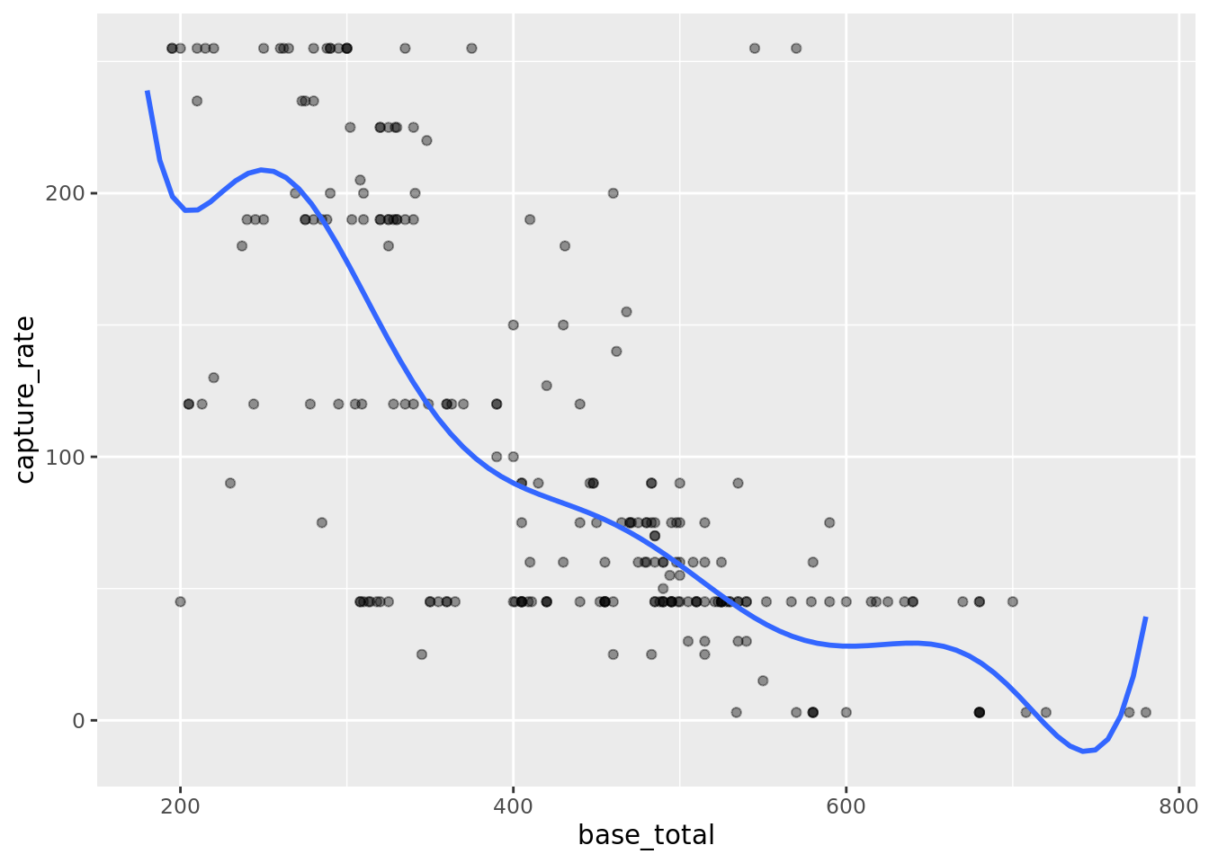
Do you notice any issue here? Looks like the model would predict negative values for capture_rate for some base_total values. How could we modify the function so this would happen? How would it help with prediction error?
7.3 Step Function
Training step functions can be difficult in R because you are turning a continuous variable into a factor variable and maintaining the factor structure across splits and folds is a pain. The new tidymodels approach to statistical/machine learning with R makes this much easier and students should consider gaining knowledge about this suite of packages. These were not quite ready for us at the beginning of this class or we would have been using tidymodels in this class. The next version of this class will use these packages.
For now we will simply create the cuts for the step functions on the entire dataset before splitting. This is not best practice though. We don’t ever want to use test data information to inform the model building process. By using all the data to form the cuts we are using the this information. The ISLwR book avoided this issue by not demonstrating how to tune a step function (at least not at scale).
# add pre cut variable options
pokemon_with_cuts <- pokemon_dat %>%
  select(capture_rate, base_total) %>%
  mutate(
    bt_cut2 = cut(base_total, 2),
    bt_cut3 = cut(base_total, 3),
    bt_cut4 = cut(base_total, 4),
    bt_cut5 = cut(base_total, 5),
    bt_cut6 = cut(base_total, 6),
    bt_cut7 = cut(base_total, 7),
    bt_cut8 = cut(base_total, 8),
    bt_cut9 = cut(base_total, 9),
    bt_cut10 = cut(base_total, 10),
    bt_cut11 = cut(base_total, 11)
  )
Need a new split with the newly added cut variables included.
pokemon_cut_splits_info <- pokemon_with_cuts %>%
  initial_split(prop = 0.70)

pokemon_cut_splits <- tibble(
  train = pokemon_cut_splits_info %>% training() %>% list(),
  test = pokemon_cut_splits_info %>% testing() %>% list()
)
We can now tune the step function.
# set up models (formulas)
step_models <- tibble(
  fmla = str_c("capture_rate ~ bt_cut", 2:11),
  model_name = str_c("steps ", 2:11)
) %>%
  mutate(
    fmla = map(fmla, as.formula)
  )

# model tuning --- finding best num of steps
pokemon_cv <- pokemon_cut_splits %>%
  pluck("train", 1) %>%
  modelr::crossv_kfold(10, id = "fold") %>%
  crossing(step_models) %>%
  mutate(
    model_fit = map2(fmla, train, lm),
    fold_mse  = map2_dbl(model_fit, test, modelr::mse)
  )

# display cv test mse selecting best num of steps
pokemon_cv %>%
  group_by(model_name) %>%
  summarise(
    test_mse = mean(fold_mse)
  ) %>%
  mutate(
    # added percent diff with min test_mse to aid in comparison
    pct_diff = 100 * (test_mse - min(test_mse))/min(test_mse)
  ) %>%
  arrange(test_mse)
## # A tibble: 10 x 3
## model_name test_mse pct_diff
## <chr> <dbl> <dbl>
## 1 steps 11 2615. 0
## 2 steps 6 2620. 0.185
## 3 steps 10 2627. 0.435
## 4 steps 9 2650. 1.33
## 5 steps 7 2668. 2.01
## 6 steps 8 2880. 10.1
## 7 steps 5 2898. 10.8
## 8 steps 3 2941. 12.4
## 9 steps 4 3013. 15.2
## 10 steps 2 4140. 58.3Looks like we should a step function with 6, 7, 9, 10, or 11 steps. We could test all 5 on the model comparison data set or we could go with the simplest and most complicated. We will go with the latter.
# which is actually best
pokemon_step_fits <- step_models %>%
  filter(model_name %in% c("steps 6", "steps 11")) %>%
  crossing(pokemon_cut_splits) %>%
  mutate(
    model_fit = map2(fmla, train, lm),
    test_mse  = map2_dbl(model_fit, test, modelr::mse)
  )

# test error calc
target_var <- pokemon_cut_splits_info %>%
  testing() %>%
  pull(capture_rate) %>%
  var()

pokemon_step_fits %>%
  mutate(prop_explained = 1 - test_mse/target_var) %>%
  select(model_name, test_mse, prop_explained) %>%
  arrange(test_mse)
## # A tibble: 2 x 3
## model_name test_mse prop_explained
## <chr> <dbl> <dbl>
## 1 steps 11 2769. 0.493
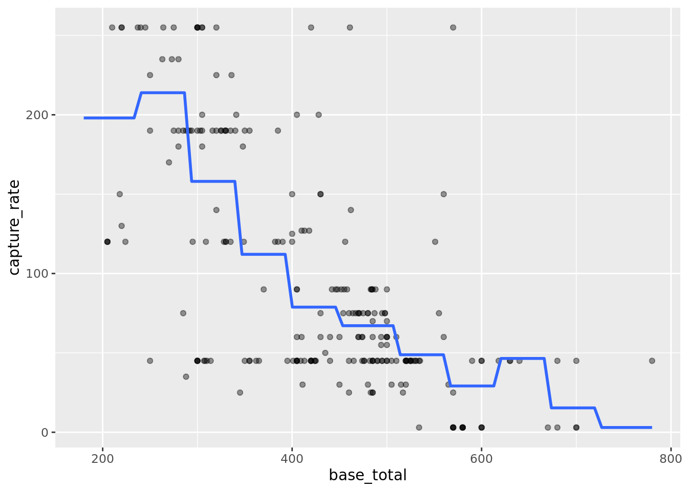
## 2 steps 6 2891. 0.471Looks like the step function with 11 steps is our winner. Let’s plot it.
# plot the fits
pokemon_cut_splits_info %>%
  testing() %>%
  ggplot(aes(base_total, capture_rate)) +
    geom_point(alpha = 0.4) +
    geom_smooth(
      data = pokemon_cut_splits_info %>% training(),
      method = "lm",
      formula = "y ~ cut(x, 11)",
      se = FALSE
    )
7.4 Splines
7.5 GAMs
The Complete Pokémon Dataset, Rounak Banik, https://www.kaggle.com/rounakbanik/pokemon. Scraped from https://serebii.net/↩