
8 Lab: Decision Trees
This is a modified version of the Lab: Decision Trees section of chapter 8 from Introduction to Statistical Learning with Application in R (ISLR). This version differs from the ISLR lab in two ways. First, it skips the process of fitting individual trees, since that is less common in data science. Second, it uses tidyverse techniques and methods that will allow for scalability and a more efficient data analytic pipeline.
To do all of this, we will need the libraries loaded below
# Data wrangling
library(tidyverse)
library(janitor)
library(modelr)
library(rsample)

# For random forests
library(ranger)
library(vip)
library(pdp)

# For boosted models
library(xgboost)
8.1 Data Preparation
For this lab we will use the Carseats data. Our outcome will be whether sales are high (i.e., > 8) or not:
# Load data
carseats <- read_csv("data/Carseats.csv") %>% # read in data
  clean_names() %>%
  mutate(high = as.factor(ifelse(sales <= 8, "No", "Yes")), # add column for 'high' sales
         high = fct_relevel(high, "Yes")) %>% # Make sure class 'Yes' is what's being predicted
  mutate_if(is.character, factor) # clean up factors
We can break this dataset into training and test data:
set.seed(15431)

carseats_split_info <- carseats %>%
  initial_split(prop = 0.7)

carseats_split <- tibble(
  train = carseats_split_info %>% training() %>% list(),
  test = carseats_split_info %>% testing() %>% list()
)
8.2 Bagging & Random Forests for Classification
Bagging and random forests are really two sides of the same coin. They both involve taking bootstrap samples of the training data and fitting a tree to each sample. The main difference between them is that for each tree fit using bagging, all of the \(p\) predictors in the data are considered for each split. Conversely, in the random forest, only a random sample \(m < p\) predictors are considerd for each split.
We can use the same function ranger() from the ranger library for both bagging and random forests. The ranger() function takes a formula and data argument, much like other functions in R (e.g., lm()). In addition, ranger() takes an argument mtry, which specifies the number of predictors \(m\) considered for each split. For example, if there are 20 predictors, calling ranger() with mtry = 20 is the same thing as bagging. But setting mtry = 10 is a random forest that considers a random sample of 10 predictors for each split in each tree.
Our first random forest will involve a classification problem: we wish to predict whether a store has high sales of carseats (i.e., sales > 8). The outcome we are interested is the high column, which we defined in the data preparation section.
To help us test our fitted models, we will write a helper function to get the misclassification rate on a test set given a fitted model:
# helper function to get misclass rate from a ranger object
#' @name misclass_ranger
#' @param model ranger object, a fitted random forest
#' @param test tibble/resample object, a test set
#' @param outcome string, indicates the outcome variable in the data
#' @returns misclassification rate of the model on the test set
misclass_ranger <- function(model, test, outcome){

  # Check if test is a tibble
  if(!is_tibble(test)){
    test <- test %>% as_tibble()
  }

  # Make predictions
  preds <- predict(model, test)$predictions

  # Compute misclass rate
  misclass <- mean(test[[outcome]] != preds)

  return(misclass)

}
Now we’re ready to start fitting and testing random forests. The code below uses several different values of mtry from 1 up to 10, where 10 is the total number of predictors in this prediction problem (since we exclude sales).
carseats_rf_class <- carseats_split %>%
  crossing(mtry = 1:(ncol(carseats) - 2)) %>% # list all mtry values
  # Fit the model for each mtry value
  mutate(model = map2(.x = train, .y = mtry,
                      .f = function(x, y) ranger(high ~ . - sales, # exlcude sales
                                                 mtry = y,
                                                 data = x,
                                                 splitrule = "gini", # Use the gini index
                                                 importance = "impurity")), # Record impurity at each split
         # Get the train, test and OOB misclassification rates
         train_misclass = map2(model, train, misclass_ranger, outcome = "high"),
         test_misclass = map2(model, test, misclass_ranger, outcome = "high"),
         oob_misclass = map(.x = model,
                         .f = function(x) x[["prediction.error"]])
         )
Perhaps one of the first things we may want to check is how well our models perform. Below, we plot the training, test, and out-of-bag (OOB) misclassification rates as a function of mtry. What we see from the test error is that a value of mtry = 6 tends to perform fairly well. Moreover, the OOB error appears to be a pretty good proxy for the test error–at least it is a much better proxy than just the training error.
ggplot(carseats_rf_class) +
  geom_line(aes(mtry, unlist(oob_misclass), color = "OOB Error")) +
  geom_line(aes(mtry, unlist(train_misclass), color = "Training Error")) +
  geom_line(aes(mtry, unlist(test_misclass), color = "Test Error")) +
  labs(x = "mtry", y = "Misclassification Rate") +
  scale_color_manual("", values = c("purple", "blue", "red")) +
  theme_bw()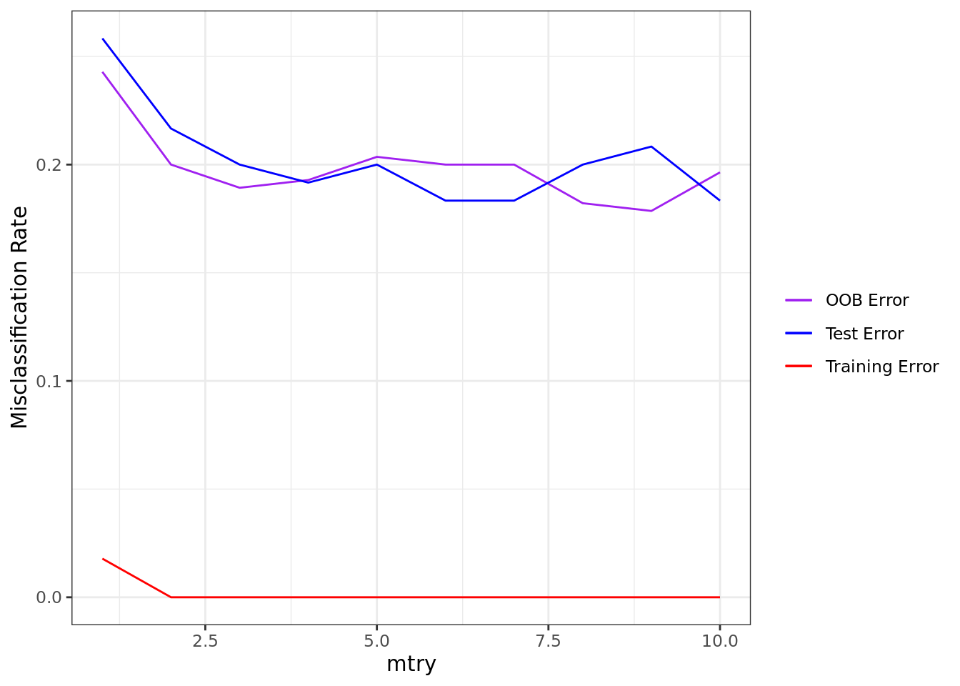
8.2.1 Variable Importance
An important aspect of these models is that while they are often viewed as “black boxes,” there are a number of ways in which we can simplify their interpretation. First, we can examine the variable importance plot, which indicates how much the inclusion of a variable improves the predictions of the model. Variable importance plots present a bar for each predictor and longer bars indicate more important predictors. Below, we see that price is the most important driver of sales, however shelf location and advertising spending are also useful.
To make variable importance plots, we can use the vip() function from the vip library. The vip() function takes a ranger object as an argument and automatically outputs the plot in the style of ggplot2.
rf_class_mtry6 = ranger(high ~ . - sales,
                        data = carseats,
                        mtry = 6,
                        importance = "impurity",
                        splitrule = "gini",
                        probability = TRUE)
vip(rf_class_mtry6)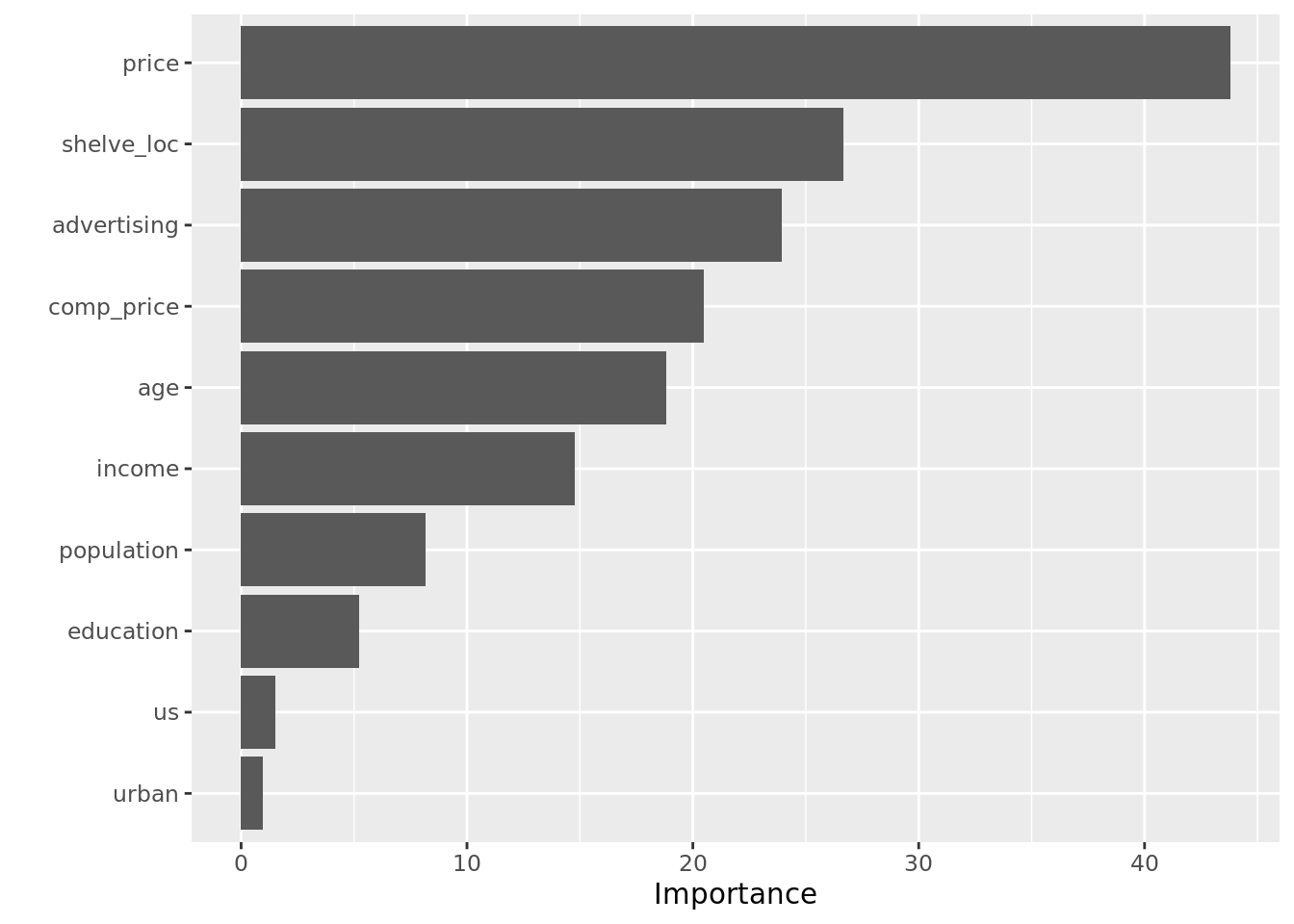
8.2.2 Partial Dependence
Another way to interpret models is through partial dependence plots. These plots show the marginal relationship between a given predictor and the outcome in the model. Below, we see a partial dependence plot between price and the probability that a store has high sales (high). In the plot, the relationship between price and high sales is relatively flat when the price is very low or very high, but it substantially increases as the price increases from $75 to $150.
Note that in order to generate this plot, we use the partial() function from the pdp library. This function takes a ranger object as an argument, as well as a string indicating the predictor variable we are interested in. Note that we can output ggplot2 graphics using the plot.engine argument.
partial(rf_class_mtry6,
        pred.var = "price",
        plot = TRUE,
        rug = TRUE,
        prob = TRUE, # Plot the raw probability
        plot.engine = "ggplot2") +
  labs(y = "High Sales", x = "Price")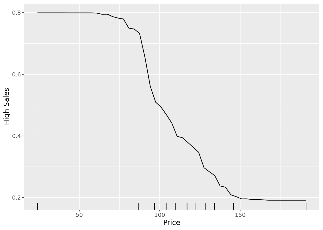
8.3 Bagging & Random Forests for Regression
A convenient aspect of decision trees is that when we move from classification to regression, the algorithm is largely unchanged. The only major change is that when the algorithm considers split rules, it uses different criteria to determine what a good split is. In regression, this criterion is usually squared errors in the terminal nodes.
In this section, we predict sales, a continuous outcome in the Carseats data. Since the algorithm is so similar to that of the classification problem in the previous section, our pipeline for workflow will remain largely the same.
Here, we define a helper function to get test MSE for our fitted models.
# helper function to get misclass rate from a ranger object
#' @name mse_ranger
#' @param model ranger object, a fitted random forest
#' @param test tibble/resample object, a test set
#' @param outcome string, indicates the outcome variable in the data
#' @returns MSE of the model on the test set
mse_ranger <- function(model, test, outcome){

  # Check if test is a tibble
  if(!is_tibble(test)){
    test <- test %>% as_tibble()
  }

  # Make predictions
  preds <- predict(model, test)$predictions

  # Compute MSE
  mse <- mean((test[[outcome]] - preds)^2)

  return(mse)

}
Now we’re ready to fit and tune some regression models. Note that the code here is nearly identical to the code from the previous section on classification.
carseats_rf_reg <- carseats_split %>%
  crossing(mtry = 1:(ncol(carseats) - 2)) %>% # tune different values of mtry
  mutate(# Fit models for each value of mtry
         model = map2(.x = train, .y = mtry,
                      .f = function(x, y) ranger(sales ~ . - high,
                                                 mtry = y,
                                                 data = x,
                                                 splitrule = "variance", # use 'variance' for regression
                                                 importance = "impurity")),
         # Get training, test, and OOB error
         train_err = map2(model, train, mse_ranger, outcome = "sales"),
         test_err = map2(model, test, mse_ranger, outcome = "sales"),
         oob_err = map(.x = model,
                       .f = function(x) x[["prediction.error"]])
         )
Again, it is usually a good idea to check our tuning. Below, we have a plot of the training, test, and OOB error versus mtry. It would appear that an mtry of about 8 works pretty well.
ggplot(carseats_rf_reg) +
  geom_line(aes(mtry, unlist(oob_err), color = "OOB Error")) +
  geom_line(aes(mtry, unlist(train_err), color = "Training Error")) +
  geom_line(aes(mtry, unlist(test_err), color = "Test Error")) +
  labs(x = "mtry", y = "MSE") +
  scale_color_manual("", values = c("purple", "red", "blue")) +
  theme_bw()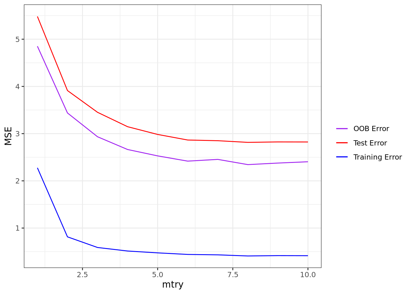
8.3.1 Variable Importance
Using our preferred mtry from above, we can begin unpacking that model. First up is the variable importance plot, courtesy of the vip() function. What we can see is that shelf location and price are the two biggest drivers of carseat sales.
rf_reg_mtry8 = ranger(sales ~ . - high,
                      data = carseats,
                      mtry = 8,
                      importance = "impurity",
                      splitrule = "variance")
vip(rf_reg_mtry8)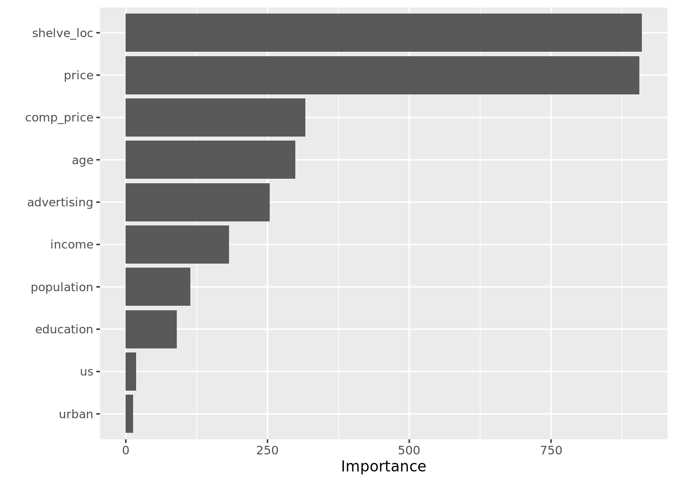
8.3.2 Partial Dependence
Again, we can examine partial dependence plots to unpack the marginal relationships between specific variables and the outcome. Consistent with the classification problem, we see a nonlinear relationship between price and sales.
partial(rf_reg_mtry8,
        pred.var = "price",
        pred.data = carseats,
        plot = TRUE,
        rug = TRUE,
        plot.engine = "ggplot2") +
  labs(y = "Sales", x = "Price")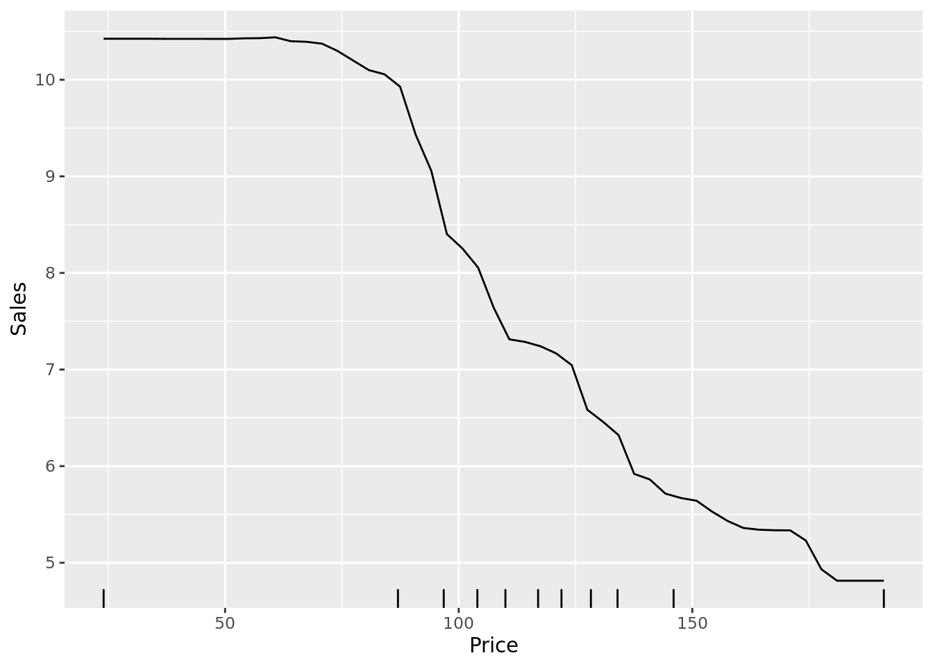
8.4 Tuning Random Forests
Random forests and bagged models have a whole host of tuning paramaters. Above, we examined the impact of one of those parameters, mtry, using a validation set approach. However, we could have also tuned the tree depth max.depth or the number of trees num.trees. Usually, tuning mtry will make the biggest impact, but it is always a good idea to tune other parameters, just to make sure. Note that if you are working with a dataset that is large enough to render cross validation too time-consuming, you can tune your models on the fly using the OOB error!
Take some time here to figure out how to alter the code above so that it incorporates \(k\)-fold cross validation. Where would you fold the data? How would you need to change the helper or in-line functions?
8.5 Boosted Models and Helper Functions
Boosted models are another powerful predictive tool. In this lab, we’ll use the xgboost library to train and test models. An important facet of the functions in this library is that they accept a specific data structure called a DMatrix. Thus, it is useful to have a helper function to convert our tibbles into DMatrix format.
# helper function
#' @name xgb_matrix
#' @param dat tibble, dataset
#' @param outcome string, indicates the outcome variable in the data
#' @param exclude_vars string (or list of strings) to indicate variables to exclude
#' @returns MSE of the model on the test set
xgb_matrix <- function(dat, outcome, exclude_vars){

  # Sanitize input: check that dat is a tibble
  if(!is_tibble(dat)){

    dat <- as_tibble(dat)

  }

  # Sanitize input: check that data has factors, not characters
  dat_types <- dat %>% map_chr(class)

  outcome_type <- class(dat[[outcome]])

  if("character" %in% dat_types){

    # If we need to re-code, leave that outside of the function
    print("You must encode characters as factors.")
    return(NULL)

  } else {

    # If we're doing binary outcomes, they need to be 0-1
    if(outcome_type == "factor" & nlevels(dat[[outcome]]) == 2){
      tmp <- dat %>% select(outcome) %>% onehot::onehot() %>% predict(dat)
      lab <- tmp[,1]
    } else {
      lab <- dat[[outcome]]
    }

    # Make our DMatrix
    mat <- dat %>% dplyr::select(-outcome, -all_of(exclude_vars)) %>% # encode on full boston df
      onehot::onehot() %>% # use onehot to encode variables
      predict(dat) # get OHE matrix

    return(xgb.DMatrix(data = mat,
                       label = lab))

  }

}
It will also be useful to have a helper function to get our training and test error. The predict.xg.Booster() function assumes that the data you feed it is a DMatrix, so we’ll have to make sure your test data is in that format. Instead of writing two functions to get our test error, here we’ll see if we can get away with just writing one:
# helper function
#' @name xg_error
#' @param model xgb object, a fitted boosted model
#' @param test_mat DMatrix, a test set
#' @param metric string (either "mse" or "misclass"), indicates the error metric
#' @returns MSE/misclass rate of the model on the test set
xg_error <- function(model, test_mat, metric = "mse"){

  # Get predictions and actual values
  preds = predict(model, test_mat)
  vals = getinfo(test_mat, "label")

  if(metric == "mse"){

    # Compute MSE if that's what we need
    err <- mean((preds - vals)^2)

  } else if(metric == "misclass") {

    # Otherwise, get the misclass rate
    err <- mean(preds != vals)

  }

  return(err)
}
8.6 Boosted Models for Classification
Now we’re ready to fit some boosted models. As with the random forests, we’ll use a validation set approach to tune the learning rate. The function we use to fit models is xgb.train() which takes several arguments, including data (which must be a DMatrix) and a list of parameters. Within that list of parameters, the eta argument is the learning rate. Note that we can chance the objective function
carseats_xg_class <- carseats_split %>%
   crossing(learn_rate = 10^seq(-10, -.1, length.out = 20)) %>% # tune the learning rate
   mutate(# Build xgb Dmatrices for training and test set
          train_mat = map(train, xgb_matrix, outcome = "high", exclude_vars = "sales"),
          test_mat = map(test, xgb_matrix, outcome = "high", exclude_vars = "sales"),
          # Fit models to each learning rate
          xg_model = map2(.x = train_mat, .y = learn_rate,
                         .f = function(x, y) xgb.train(params = list(eta = y, # set learning rate
                                                                     depth = 10, # tree depth, can tune
                                                                     objective = "multi:softmax", # output labels
                                                                     num_class = 2), # binary class problem
                                                       data = x,
                                                       nrounds = 500, # 500 trees, can be tuned
                                                       silent = TRUE)),
         # Get training and test error
         xg_train_misclass = map2(xg_model, train_mat, xg_error, metric = "misclass"),
         xg_test_misclass = map2(xg_model, test_mat, xg_error, metric = "misclass")
    )
Here, we can check how the learning rate affected the misclassification rate on the test set. It would appear that a really small learning rate (<0.01) works best.
# Plot test error
ggplot(carseats_xg_class) +
  geom_line(aes(learn_rate, unlist(xg_test_misclass)))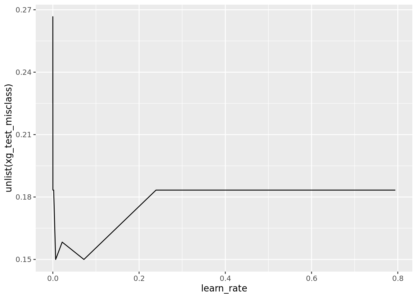
We can compute similar interpretive diagnostics on this model, including variable importance and partial dependence plots:
xg_class_mod <- carseats_xg_class %>%
  arrange(unlist(xg_test_misclass)) %>%
  pluck("xg_model", 1)

vip(xg_class_mod)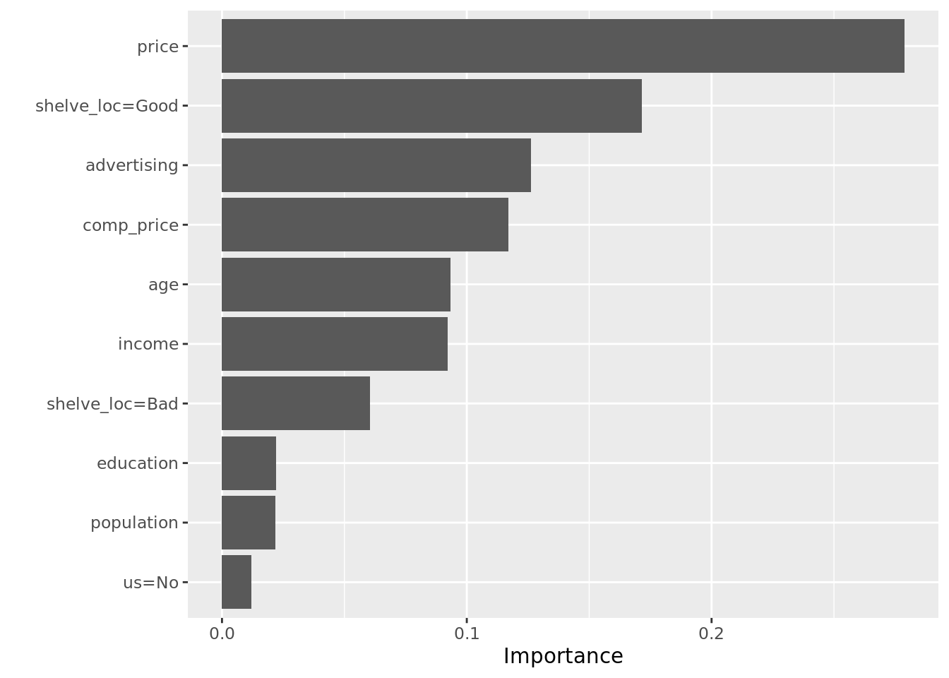
8.7 Boosted Models for Regression
The procedure for fitting and tuning boosted models for regression will be nearly identical to the one we used for classification above. The key difference is the objective function, and the matrices we create.
carseats_xg_reg <- carseats_split %>%
   crossing(learn_rate = 10^seq(-10, -.1, length.out = 20)) %>% # tune the learning rate
   mutate(# Build xgb Dmatrices for training and test set
          train_mat = map(train, xgb_matrix, outcome = "sales", exclude_vars = "high"),
          test_mat = map(test, xgb_matrix, outcome = "sales", exclude_vars = "high"),
          # Train xgb models for each learning rate
          xg_model = map2(.x = train_mat, .y = learn_rate,
                          .f = function(x, y) xgb.train(params = list(eta = y,
                                                                      depth = 10, # tree depth, can tune
                                                                      objective = "reg:squarederror"), # minimize MSE
                                                        data = x,
                                                        nrounds = 500, # fit 500 trees, can tune
                                                        silent = TRUE)),
          # Get training and test error
          xg_train_mse = map2(xg_model, train_mat, xg_error, metric = "mse"),
          xg_test_mse = map2(xg_model, test_mat, xg_error, metric = "mse"))
Again, from the plot below, which shows MSE versus learning rate, a very small error rate will probably work best (given the other tuning parameters; see below)
# Plot training and test error
ggplot(carseats_xg_reg) +
  geom_line(aes(learn_rate, unlist(xg_train_mse), color = "Training Error")) +
  geom_line(aes(learn_rate, unlist(xg_test_mse), color = "Test Error")) +
  scale_color_manual("", values = c("blue", "red")) +
  labs(x = "Learning Rate", y = "MSE")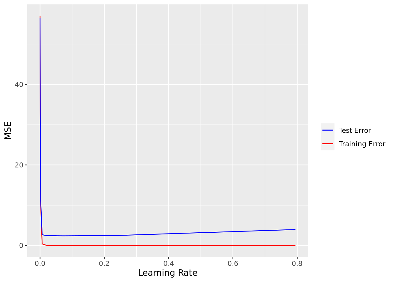
Again, we can plot the variable importance; what do you see in this plots?
# Get best model
xg_reg_mod <- carseats_xg_reg %>%
  arrange(unlist(xg_test_mse)) %>%
  pluck("xg_model", 1)

# Examine variable importance
vip(xg_reg_mod)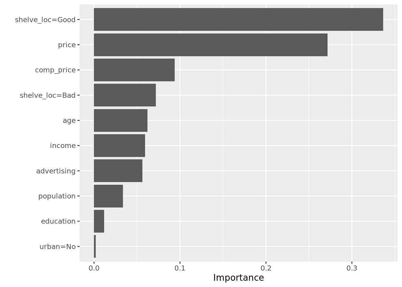
8.8 Tuning Boosted Models
An important thing to note is that there are a very large number of tuning parameters for boosted models, including:
nroundsthe number of trees fitetathe learning rategamma,max_depth,min_child_weightwhich each govern tree depth in different wayscolsample_bytreewhich allows you to grow trees by randomly selecting subsets of predictors for each split rule (like you would in a random forest)
Typically, tuning nrounds and eta will improve your model the most, but it is usually a good idea to check other parameters.
Finally, while we used a validation set approach to tuning in this lab, a better approach would use cross-validation. Take some time now to think about how you would tweak the code in this lab to incorporate a cross-validation loop. Where would you fold the data (i.e., which line of code)? What would you need to change about the helper and in-line functions?