
6 Lab: Linear Model Selection and Regularization
This is a modified version of Lab 1: Subset Selection Methods, Lab 2: Ridge Regression and the Lasso, and Lab 3: PCR and PLS Regression labs from chapter 6 of Introduction to Statistical Learning with Application in R. This version uses tidyverse techniques and methods that will allow for scalability and a more efficient data analytic pipeline.
We will need the packages loaded below.
# Load packages
library(tidyverse)
library(modelr)
library(janitor)
library(skimr)
library(leaps) # best subset selection
library(glmnet) # ridge & lasso
library(glmnetUtils) # improves working with glmnet
library(pls) # pcr and pls
Since we will be making use of validation set and cross-validation techniques to build and select models we should set our seed to ensure the analyses and procedures being performed are reproducible. Readers will be able to reproduce the lab results if they run all code in sequence from start to finish — cannot run code chucks out of order. Setting the seed should occur towards the top of an analytic script, say directly after loading necessary packages.
# Set seed
set.seed(27182) # Used digits from e
6.1 Data Setup
We will be using the Hitters dataset from the ISLR library. Take a moment and inspect the codebook — ?ISLR::Hitters. Our goal will be to predict salary from the other available predictors.
hitter_dat <- read_csv("data/Hitters.csv") %>%
  clean_names() %>%
  rename(c_rbi = crbi) %>%
  mutate_at(vars(league, division, new_league), factor)
Let’s skim the data to make sure it has been encoded correctly and quickly inspect it for other potential issues such as missing data.
hitter_dat %>%
  skim_without_charts()
## ── Data Summary ────────────────────────
## Values
## Name Piped data
## Number of rows 322
## Number of columns 21
## _______________________
## Column type frequency:
## character 1
## factor 3
## numeric 17
## ________________________
## Group variables None
##
## ── Variable type: character ────────────────────────────────────────────────────────────────────────
## skim_variable n_missing complete_rate min max empty n_unique whitespace
## 1 name 0 1 7 17 0 322 0
##
## ── Variable type: factor ───────────────────────────────────────────────────────────────────────────
## skim_variable n_missing complete_rate ordered n_unique top_counts
## 1 league 0 1 FALSE 2 A: 175, N: 147
## 2 division 0 1 FALSE 2 W: 165, E: 157
## 3 new_league 0 1 FALSE 2 A: 176, N: 146
##
## ── Variable type: numeric ──────────────────────────────────────────────────────────────────────────
## skim_variable n_missing complete_rate mean sd p0 p25 p50 p75 p100
## 1 at_bat 0 1 381. 153. 16 255. 380. 512 687
## 2 hits 0 1 101. 46.5 1 64 96 137 238
## 3 hm_run 0 1 10.8 8.71 0 4 8 16 40
## 4 runs 0 1 50.9 26.0 0 30.2 48 69 130
## 5 rbi 0 1 48.0 26.2 0 28 44 64.8 121
## 6 walks 0 1 38.7 21.6 0 22 35 53 105
## 7 years 0 1 7.44 4.93 1 4 6 11 24
## 8 c_at_bat 0 1 2649. 2324. 19 817. 1928 3924. 14053
## 9 c_hits 0 1 718. 654. 4 209 508 1059. 4256
## 10 c_hm_run 0 1 69.5 86.3 0 14 37.5 90 548
## 11 c_runs 0 1 359. 334. 1 100. 247 526. 2165
## 12 c_rbi 0 1 330. 333. 0 88.8 220. 426. 1659
## 13 c_walks 0 1 260. 267. 0 67.2 170. 339. 1566
## 14 put_outs 0 1 289. 281. 0 109. 212 325 1378
## 15 assists 0 1 107. 137. 0 7 39.5 166 492
## 16 errors 0 1 8.04 6.37 0 3 6 11 32
## 17 salary 59 0.817 536. 451. 67.5 190 425 750 2460We see there is some missing data/values which are all contained in the response variable salary. There isn’t much we could do here unless we would want to do some research ourselves and see if we can find them somewhere else. We will remove them from our dataset. Note that we could still produce predicted salaries for these players, but we just won’t be able to determine if the predictions are any good.
hitter_dat <- hitter_dat %>% na.omit()We will be implementing model selection later in this lab and we have a choice which impacts how we need to handle the dataset. We could opt to use \(C_p\), \(BIC\), or \(R^2_{adj}\) or we could use validation set or cross-validation approaches. Remember that \(C_p\), \(BIC\), or \(R^2_{adj}\) are essentially methods that indirectly estimate test \(MSE\) while validation set or cross-validation approaches provide direct estimates of test \(MSE\). The indirect approaches require many assumptions that may not be tenable and they use the entire dataset. We prefer the direct approaches to estimating test \(MSE\) because they are more flexible and computational limitations are no longer a barrier.
# Test set for comparing candidate models -- selecting final model
hitter_mod_comp_dat <- hitter_dat %>% sample_frac(0.15)

# Train set for candidate model building
hitter_mod_bldg_dat <- hitter_dat %>% setdiff(hitter_mod_comp_dat)
6.2 Subset Selection Methods
## Helper functions

# Get predicted values using regsubset object
predict_regsubset <- function(object, fmla , new_data, model_id)
{
  # Not a dataframe? -- handle resample objects/k-folds
  if(!is.data.frame(new_data)){
    new_data <- as_tibble(new_data)
  }

  # Get formula
  obj_formula <- as.formula(fmla)

  # Extract coefficients for desired model
  coef_vector <- coef(object, model_id)

  # Get appropriate feature matrix for new_data
  x_vars <- names(coef_vector)
  mod_mat_new <- model.matrix(obj_formula, new_data)[ , x_vars]

  # Get predicted values
  pred <- as.numeric(mod_mat_new %*% coef_vector)

  return(pred)
}

# Calculate test MSE on regsubset objects
test_mse_regsubset <- function(object, fmla , test_data){

  # Number of models
  num_models <- object %>% summary() %>% pluck("which") %>% dim() %>% .[1]

  # Set up storage
  test_mse <- rep(NA, num_models)

  # observed targets
  obs_target <- test_data %>%
    as_tibble() %>%
    pull(!!as.formula(fmla)[[2]])

  # Calculate test MSE for each model class
  for(i in 1:num_models){
    pred <- predict_regsubset(object, fmla, test_data, model_id = i)
    test_mse[i] <- mean((obs_target - pred)^2)
  }

  # Return the test errors for each model class
  tibble(model_index = 1:num_models,
         test_mse    = test_mse)
}
# Best susbset: use 10-fold CV to select optimal number of variables
hitter_bestsubset_cv <- hitter_mod_bldg_dat %>%
crossv_kfold(10, id = "folds") %>%
mutate(
fmla = "salary ~ . -name",
model_fits = map2(fmla, train,
~ regsubsets(as.formula(.x), data = .y, nvmax = 19)),
model_fold_mse = pmap(list(model_fits, fmla ,test), test_mse_regsubset)
)
# Forward selection: use 10-fold CV to select optimal number of variables
hitter_fwd_cv <- hitter_mod_bldg_dat %>%
crossv_kfold(10, id = "folds") %>%
mutate(
fmla = "salary ~ . -name",
model_fits = map2(fmla, train,
~ regsubsets(as.formula(.x), data = .y, nvmax = 19, method = "forward")),
model_fold_mse = pmap(list(model_fits, fmla ,test), test_mse_regsubset)
)
# Backward selection: use 10-fold CV to select optimal number of variables
hitter_back_cv <- hitter_mod_bldg_dat %>%
crossv_kfold(10, id = "folds") %>%
mutate(
fmla = "salary ~ . -name",
model_fits = map2(fmla,
train,
~ regsubsets(as.formula(.x), data = .y, nvmax = 19, method = "backward")),
model_fold_mse = pmap(list(model_fits, fmla ,test), test_mse_regsubset)
)Results for best subset search.
# Plot test MSE (exhaustive search)
hitter_bestsubset_cv %>%
  unnest(model_fold_mse) %>%
  group_by(model_index) %>%
  summarise(test_mse = mean(test_mse)) %>%
  ggplot(aes(model_index, test_mse)) +
    geom_line()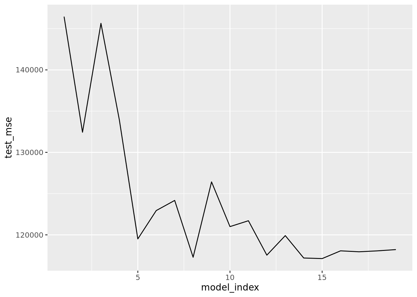
# Plot test MSE (exhaustive search)
hitter_bestsubset_cv %>%
  unnest(model_fold_mse) %>%
  group_by(model_index) %>%
  summarise(test_mse = mean(test_mse)) %>%
  arrange(test_mse)
## # A tibble: 19 x 2
## model_index test_mse
## <int> <dbl>
## 1 15 117122.
## 2 14 117193.
## 3 8 117286.
## 4 12 117538.
## 5 17 117947.
## 6 18 118060.
## 7 16 118062.
## 8 19 118214.
## 9 5 119508.
## 10 13 119908.
## 11 10 121000.
## 12 11 121711.
## 13 6 122946.
## 14 7 124173.
## 15 9 126421.
## 16 2 132444.
## 17 4 133917.
## 18 3 145646.
## 19 1 146460.Results for best foward selection search.
# Plot test MSE (forward search)
hitter_fwd_cv %>%
  unnest(model_fold_mse) %>%
  group_by(model_index) %>%
  summarise(test_mse = mean(test_mse)) %>%
  ggplot(aes(model_index, test_mse)) +
    geom_line()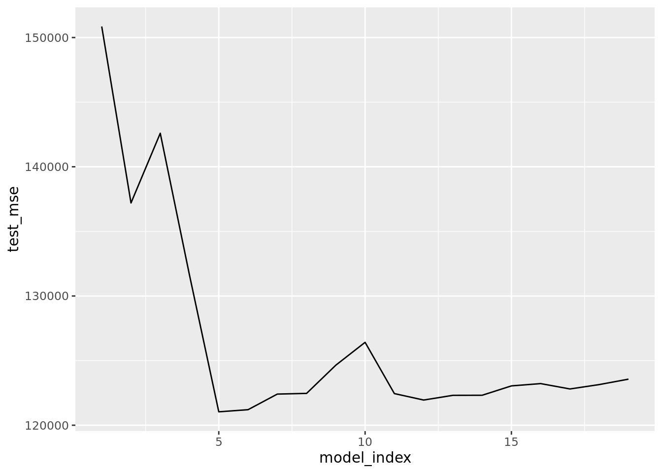
# Plot test MSE (forward search)
hitter_fwd_cv %>%
  unnest(model_fold_mse) %>%
  group_by(model_index) %>%
  summarise(test_mse = mean(test_mse)) %>%
  arrange(test_mse)
## # A tibble: 19 x 2
## model_index test_mse
## <int> <dbl>
## 1 5 121038.
## 2 6 121203.
## 3 12 121949.
## 4 13 122314.
## 5 14 122320.
## 6 7 122411.
## 7 11 122449.
## 8 8 122463.
## 9 17 122807.
## 10 15 123045.
## 11 18 123146.
## 12 16 123221.
## 13 19 123566.
## 14 9 124648.
## 15 10 126415.
## 16 4 131604.
## 17 2 137200.
## 18 3 142593.
## 19 1 150856.Results for best backward selection search.
# Plot test MSE (backward search)
hitter_back_cv %>%
  unnest(model_fold_mse) %>%
  group_by(model_index) %>%
  summarise(test_mse = mean(test_mse)) %>%
  ggplot(aes(model_index, test_mse)) +
    geom_line()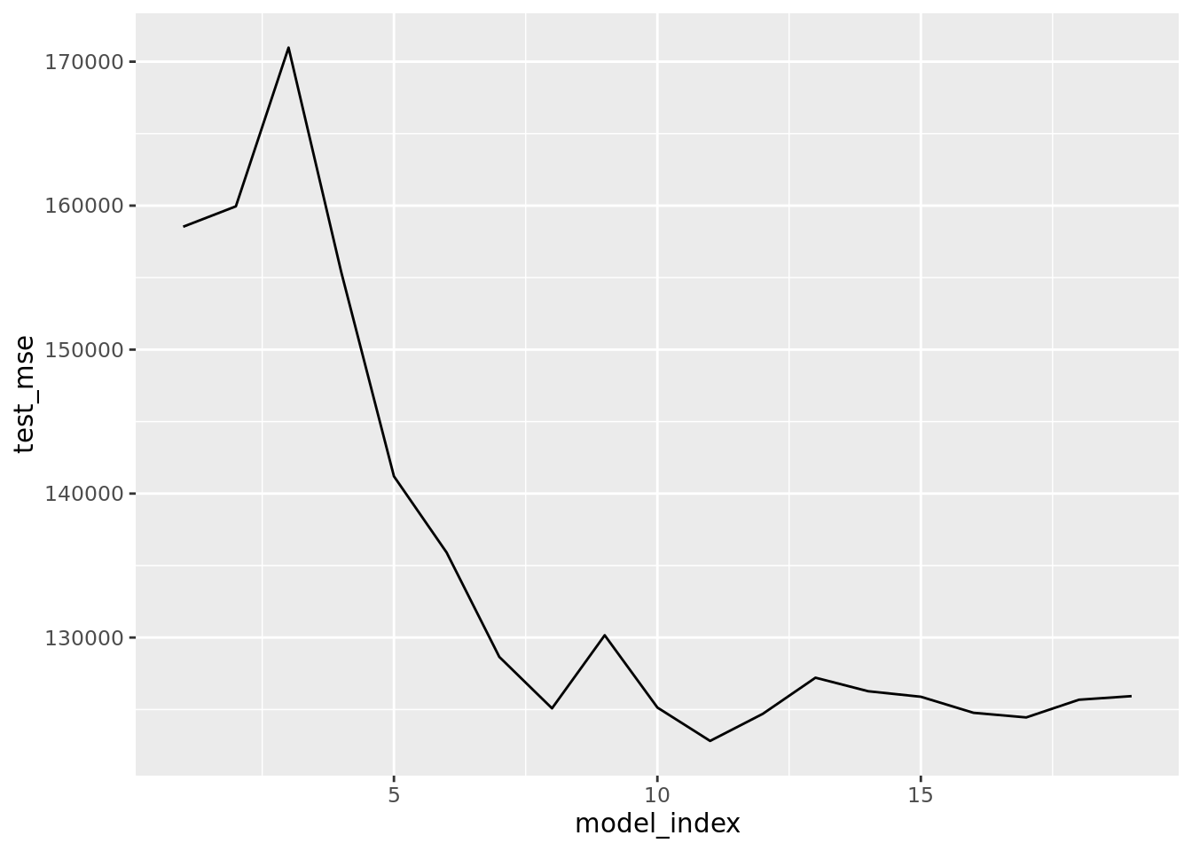
# Table test MSE (backward search)
hitter_back_cv %>%
  unnest(model_fold_mse) %>%
  group_by(model_index) %>%
  summarise(test_mse = mean(test_mse)) %>%
  arrange(test_mse)
## # A tibble: 19 x 2
## model_index test_mse
## <int> <dbl>
## 1 11 122819.
## 2 17 124451.
## 3 12 124701.
## 4 16 124772.
## 5 8 125083.
## 6 10 125138.
## 7 18 125681.
## 8 15 125887.
## 9 19 125931.
## 10 14 126270.
## 11 13 127210.
## 12 7 128654.
## 13 9 130159.
## 14 6 135905.
## 15 5 141200.
## 16 4 155383.
## 17 1 158537.
## 18 2 159953.
## 19 3 170977.The best subset (exhaustive) method suggests using a model with 8 predictors, forward selection method suggets a model with 5 or 6 predicotrs, and the backward selection method suggest a model with 8 predictors. Now implement each selection method on the entirety of hitter_mod_bldg_dat and extract the best model that uses the indicated number of predictors. These will be 3 of our candidate models.
hitter_regsubsets <- tibble(
  train = hitter_mod_bldg_dat %>% list(),
  test  = hitter_mod_comp_dat %>% list()
  ) %>%
  mutate(
    best_subset = map(train, ~ regsubsets(salary ~ . -name,
                                          data = .x , nvmax = 19)),
    fwd_selection_5 = map(train, ~ regsubsets(salary ~ . -name,
                                              data = .x, nvmax = 19,
                                              method = "forward")),
    fwd_selection_6 = map(train, ~ regsubsets(salary ~ . -name,
                                              data = .x, nvmax = 19,
                                              method = "forward")),
    back_selection = map(train, ~ regsubsets(salary ~ . -name,
                                             data = .x, nvmax = 19,
                                             method = "backward"))
    ) %>%
  pivot_longer(cols = c(-test, -train), names_to = "method", values_to = "fit")
You’ll note that backward and best subset methods settled on models having 8 predictors. It is possible that they end up producing the same same model (picking the same 8 predictors). We are probably also generally interested to see which predictors each model is using regardless of method we used. Let’s take a look at the estimated coefficients for these four models.
# Inspect/compare model coefficients
hitter_regsubsets %>%
  # extract fits
  pluck("fit") %>%
  # first input is fits; second is model info to extract
  map2(c(8, 5, 6, 8), ~ coef(.x, id = .y)) %>%
  map2(c("best", "fwd_05", "fwd_06", "back"), ~ enframe(.x, value = .y)) %>%
  reduce(full_join) %>%
  knitr::kable(digits = 3)
## Joining, by = "name"
## Joining, by = "name"
## Joining, by = "name"| name | best | fwd_05 | fwd_06 | back |
|---|---|---|---|---|
| (Intercept) | 192.149 | 160.808 | 156.443 | 192.149 |
| at_bat | -2.549 | -1.934 | -2.271 | -2.549 |
| hits | 8.162 | 8.326 | 8.585 | 8.162 |
| walks | 6.217 | NA | 3.191 | 6.217 |
| c_runs | 0.750 | NA | NA | 0.750 |
| c_rbi | 0.565 | 0.702 | 0.669 | 0.565 |
| c_walks | -0.929 | NA | NA | -0.929 |
| divisionW | -140.506 | -139.429 | -138.490 | -140.506 |
| put_outs | 0.297 | 0.315 | 0.295 | 0.297 |
The table above indicates that the best subset and backwards method selected the same model. We also see that the models selected by the forwards method use predictors that are all present in the other model. That is, the models are just constrained versions of the larger model selected by the other methods.
6.3 Ridge Regression & the Lasso
The glmnet package allows users to fit elastic net regressions which includes ridge regression (alpha = 0) and the lasso (alpha =1). Unfortunately the package does not use our familiar formula syntax, y ~ x. It requires the user to encode their data such that the penalized least squares algorithm can be applied. Both lm() and glm() also require the data to be correctly encoded for the least squares algorithm to work but this is done automatically within those functions by using the model.matrix() which takes the inputted formula and appropriately re-encodes the data for the least squares algorithm. glmnet requires the user to use model.matrix() themselves. Wouldn’t it be nice if the glmnet functions did this automatically just like lm() and glm()? Fortunately there is the glmnetUtils package which allows us to keep on using our familiar formula interface with glmnet functions.
The tuning parameter for both ridge regression and the lasso is \(\lambda\), size of the penalty to apply in the least squares algorithm. How do we go about tuning/finding an estimate for the \(\lambda\) parameter? We call upon cross-validation techniques once again. glmnet (glmnetUtils) has a built-in function that will implement cross-validation quickly and efficiently for us. Meaning there is no need for use to use crossv_kfold(). We will be using cv.glmnet() — use ?glmnetUtils::cv.glmnet to access the correct documentation. It is the alpha argument to these functions that determine if we are using ridge regression (alpha = 0) or the lasso (alpha = 1).
Since we are in search of an adequate \(\lambda\) we need to specify a range of values to search. Much like we specified the number of predictors to search over when using regsubset() — started with 1 and went up to 19. The difference here is that \(\lambda\) can be any positive real number (size of penalty to apply). Obviously we cannot use every possible value greater than 0, so we need to setup a grid search. We could go with an automatically selected grid for \(\lambda\) or we can build our own grid. We will demonstrate both.
# lambda grid to search -- use for ridge regression (200 values)
lambda_grid <- 10^seq(-2, 10, length = 200)

# ridge regression: 10-fold cv
ridge_cv <- hitter_mod_bldg_dat %>%
  cv.glmnet(
    formula = salary ~ . - name,
    data = .,
    alpha = 0,
    nfolds = 10,
    lambda = lambda_grid
    )
The following plot displays the 200 estimated test \(MSE\) values using 10 fold cross validation. The plot indicates the minimum \(\lambda\) (left dotted line). The right dotted line corresponds to a \(\lambda\) value that would result in a more regularized model (forcing more or further shrinkage of coefficients towards zero) and is within one standard error of the minimum \(\lambda\) (model’s are not all that different in estimated test \(MSE\)). Why would we desire a more regularized model? A more regularized model will typically shift more of the prediction burden/importance to fewer predictor variables. The top of the plot displays (periodically) the number of predictors in the models and in the case of ridge regression this number is very unlikely to change since it is highly unlikely to force any of the coefficients to be exactly zero.
# Check plot of cv error
plot(ridge_cv)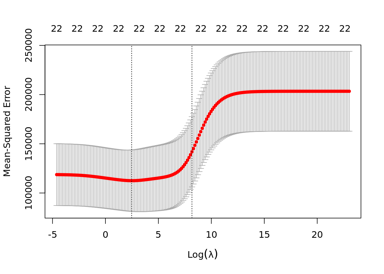
Strictly speaking the best \(\lambda\) is the one which minimizes the test error. We will extract that value to use for ridge regression. We will also extract the \(\lambda\) that is within one standard error which can help safe guard against over-fitting issues.
# ridge's best lambdas
ridge_lambda_min <- ridge_cv$lambda.min
ridge_lambda_1se <- ridge_cv$lambda.1se
Let’s get the best \(\lambda\) values for the lasso. Recall that alpha = 1 now and we will let the function select the search grid for \(\lambda\).
# lasso: 10-fold cv
lasso_cv <- hitter_mod_bldg_dat %>%
  cv.glmnet(
    formula = salary ~ . - name,
    data = .,
    alpha = 1,
    nfolds = 10
    )
Remember that the diffence between this plot and the one above. Notice The number of predictors is decreasing (top of graph) as \(\lambda\) increases. This is an important distinction between the lasso and ridge regression. Lasso forces coefficients to be zero (i.e. it is performing variable selection). For the lasso a more regularized model will result in a more parsimonious (simpler) model. For this reason it is fairly standard practice to use lambda.1se as the best \(\lambda\). This is particularly useful when theory indicates that it is likely a handful of variables are truly related to the response and the others are over-fitting to irreducible error (i.e. won’t be useful for out of sample prediction).
# Check plot of cv error
plot(lasso_cv)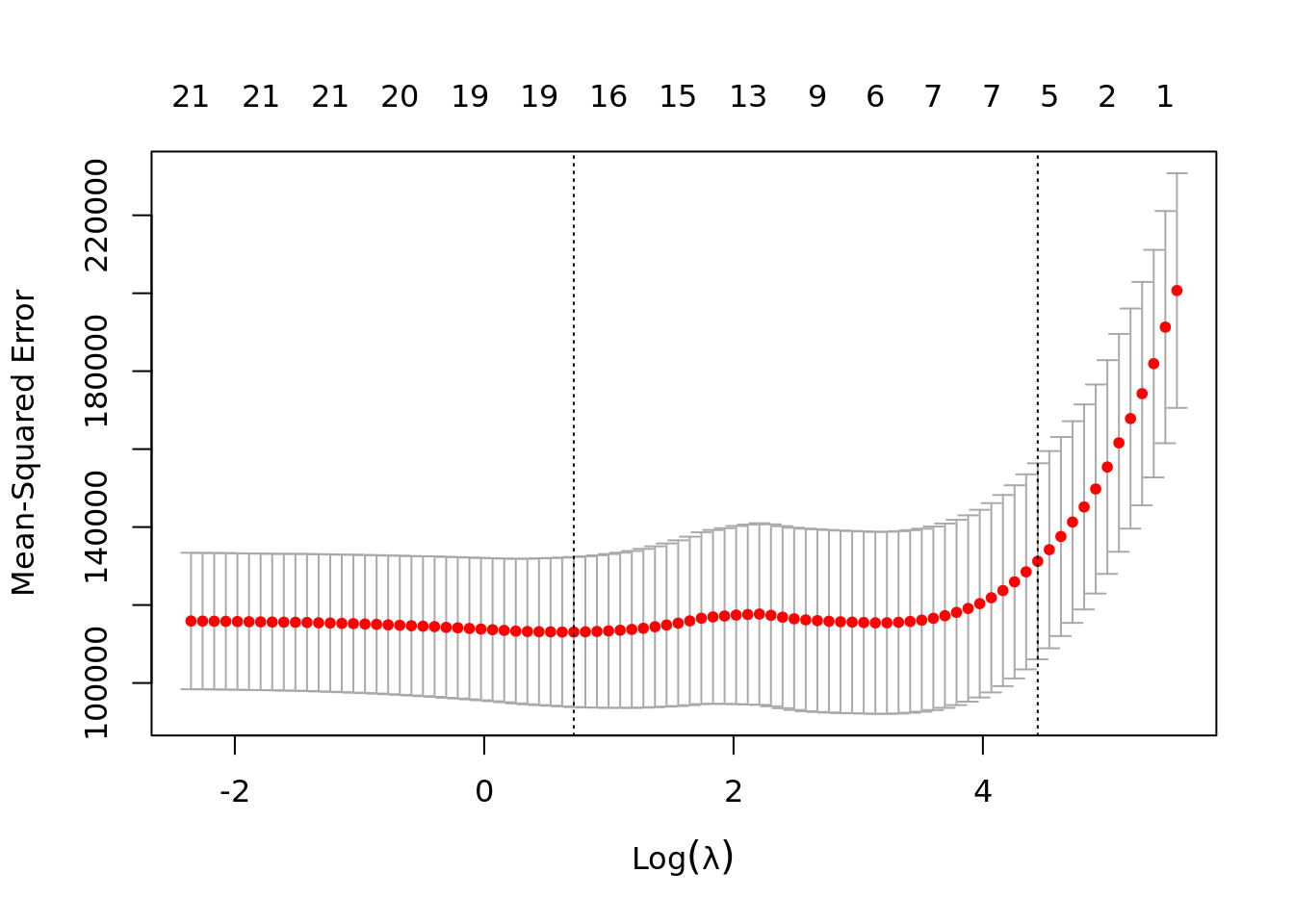
# lasso's best lambdas
lasso_lambda_1se <- lasso_cv$lambda.1se
lasso_lambda_min <- lasso_cv$lambda.min
Now that we have identified the best \(\lambda\)’s for each method we need to fit them to the entire model building dataset hitter_mod_bldg_dat. These will be our candidate models produced by ridge regression and the lasso. We do this within a tibble framework so that later we are able to calculate each model’s test error (test mse) on hitter_mod_comp_dat. This will allow us to easily compare all of our candidate models against each other in order to pick a final prediction model.
hitter_glmnet <- tibble(
  train = hitter_mod_bldg_dat %>% list(),
  test  = hitter_mod_comp_dat %>% list()
  ) %>%
  mutate(
    ridge_min = map(train, ~ glmnet(salary ~ . -name, data = .x,
                                    alpha = 0, lambda = ridge_lambda_min)),
    ridge_1se = map(train, ~ glmnet(salary ~ . -name, data = .x,
                                    alpha = 0, lambda = ridge_lambda_1se)),
    lasso_min = map(train, ~ glmnet(salary ~ . -name, data = .x,
                                    alpha = 1, lambda = lasso_lambda_min)),
    lasso_1se = map(train, ~ glmnet(salary ~ . -name, data = .x,
                                    alpha = 1, lambda = lasso_lambda_1se))
    ) %>%
  pivot_longer(cols = c(-test, -train), names_to = "method", values_to = "fit")
Let’s take a look at the coefficients for the candidate models produced by ridge regression and the lasso.
# Inspect/compare model coefficients
hitter_glmnet %>%
  pluck("fit") %>%
  map( ~ coef(.x) %>%
         as.matrix() %>%
         as.data.frame() %>%
         rownames_to_column("name")) %>%
  reduce(full_join, by = "name") %>%
  mutate_if(is.double, ~ if_else(. == 0, NA_real_, .)) %>%
  rename(ridge_min = s0.x,
         ridge_1se = s0.y,
         lasso_min = s0.x.x,
         lasso_1se = s0.y.y) %>%
knitr::kable(digits = 3)| name | ridge_min | ridge_1se | lasso_min | lasso_1se |
|---|---|---|---|---|
| (Intercept) | 128.869 | 243.584 | 111.713 | 175.101 |
| at_bat | -1.373 | 0.074 | -2.111 | NA |
| hits | 4.554 | 0.318 | 7.066 | 1.352 |
| hm_run | -5.922 | 0.788 | -2.658 | NA |
| runs | 0.517 | 0.476 | NA | NA |
| rbi | 1.621 | 0.505 | 0.265 | NA |
| walks | 3.929 | 0.586 | 4.880 | 0.382 |
| years | -14.477 | 2.362 | -14.301 | NA |
| c_at_bat | -0.007 | 0.007 | NA | NA |
| c_hits | 0.181 | 0.026 | NA | NA |
| c_hm_run | 0.616 | 0.189 | NA | NA |
| c_runs | 0.330 | 0.050 | 0.603 | 0.009 |
| c_rbi | 0.426 | 0.055 | 0.739 | 0.471 |
| c_walks | -0.474 | 0.054 | -0.662 | NA |
| leagueA | -37.974 | -2.640 | -45.825 | NA |
| leagueN | 38.034 | 2.640 | 0.000 | NA |
| divisionE | 72.204 | 18.242 | 138.364 | 4.839 |
| divisionW | -72.092 | -18.242 | NA | NA |
| put_outs | 0.302 | 0.046 | 0.301 | 0.087 |
| assists | 0.231 | 0.005 | 0.235 | NA |
| errors | -4.729 | -0.081 | -3.159 | NA |
| new_leagueA | 22.324 | -2.639 | 12.415 | NA |
| new_leagueN | -22.244 | 2.639 | 0.000 | NA |
6.4 PCR & PLS Regression
Will will be using pcr() from the pls library to implement principal component regression. Recall the purpose of PCR is to reduce the dimension of our predictor set. That is we want to find a set of \(m\) principal components (linear combinations of predictors) that we will then use in a linear regression. This is to solve the problem of having too many predictors relative to observations, especially when the number of predictors exceeds that of our observations (\(p > n\)).
Hopefully it is clear that \(m\), the number of principal components, is just a tuning parameter. Meaning we can once again turn to cross-validation techniques to pick the optimal \(m\), optimal in that we want the lowest possible test error. We can set validation = "CV" in pcr() to conduct 10-fold cross-validation by default. Note that you can control the number by specifying, for example, segments = 5 for 5-fold cross-validation.
Before we proceed to tuning the \(m\) parameter there is one more important decision to be made. Do we want to standardize each predictor variable prior to forming the principal components? This is a very important decision because forming principal components is sensitive to scale and standardizing each variable forces them to have the same scale. If we choose to standardize the predictors than we are saying they are all equally important and none should be prioritized over the other due to how it is measured. If not, we are indicating that the scale of the predictor variables is important and should be taken into account when forming principal components. In most cases we will want scale = TRUE because we will have many variables measured on many different scales with no reasonable justification to believe that the scale of the measure should be important. For example a variable such as height does not become more useful when measured in centimeters, then measured in meters.
# pcr: 10-fold cv
pcr_cv <- hitter_mod_bldg_dat %>%
  pcr(salary ~ . -name, data = ., scale = TRUE, validation = "CV")
We can use validationplot() to find the \(m\) (number of components) that corresponds to the lowest estimated test error (either reported as root mean squared error or mean squared error). The plots below indicate that 6 would be the optimal number of principal components — added a vertical line at 6 to help identify.
# Using root mean squared error
validationplot(pcr_cv)
abline(v = 7) # add vertical line at 7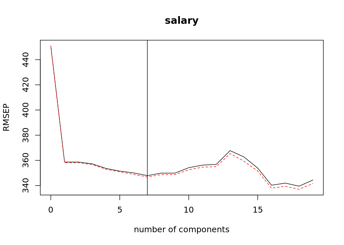
# Using mean squared error
validationplot(pcr_cv, val.type="MSEP")
abline(v = 7) # add vertical line at 7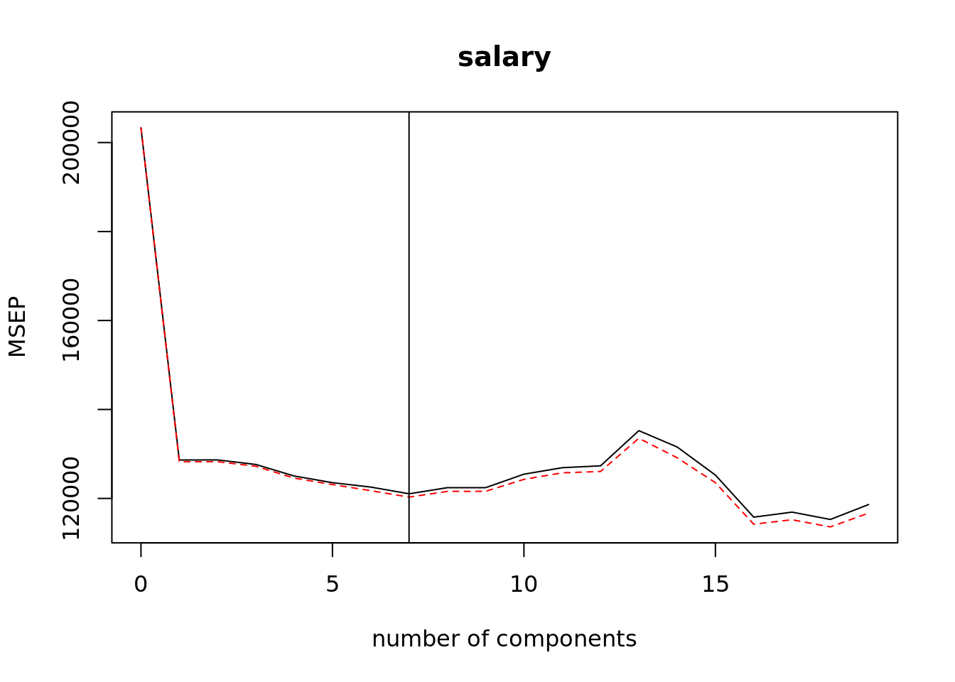
If it becomes too difficult to determine the optimal value using a validationplot() then use summary() to get a table of the values.
pcr_cv %>%
  summary()
## Data: X dimension: 224 19
## Y dimension: 224 1
## Fit method: svdpc
## Number of components considered: 19
##
## VALIDATION: RMSEP
## Cross-validated using 10 random segments.
## (Intercept) 1 comps 2 comps 3 comps 4 comps 5 comps 6 comps 7 comps 8 comps 9 comps
## CV 450.9 358.7 358.7 357.3 353.6 351.5 350.1 347.9 349.9 349.9
## adjCV 450.9 358.1 358.1 356.7 352.9 350.9 348.9 346.8 348.7 348.7
## 10 comps 11 comps 12 comps 13 comps 14 comps 15 comps 16 comps 17 comps 18 comps
## CV 354.2 356.2 356.8 367.7 362.7 353.9 340.3 341.9 339.5
## adjCV 352.5 354.6 355.0 365.4 359.4 351.5 338.0 339.4 337.0
## 19 comps
## CV 344.4
## adjCV 341.6
##
## TRAINING: % variance explained
## 1 comps 2 comps 3 comps 4 comps 5 comps 6 comps 7 comps 8 comps 9 comps 10 comps
## X 38.69 59.96 71.03 79.41 84.48 88.82 92.52 95.18 96.39 97.37
## salary 39.53 39.92 40.63 42.33 43.93 46.04 46.99 47.14 47.30 48.42
## 11 comps 12 comps 13 comps 14 comps 15 comps 16 comps 17 comps 18 comps 19 comps
## X 98.03 98.66 99.17 99.47 99.75 99.90 99.97 99.99 100.0
## salary 48.54 48.71 49.16 52.12 52.80 55.97 56.39 56.89 56.9Let’s move on to calculating the optimal \(m\) when using plsr(), partial least squares regression. Note that \(m\) stands for the number of partial least squares directions (much like the number of principal components).
# pls: 10-fold cv
pls_cv <- hitter_mod_bldg_dat %>%
  plsr(salary ~ . -name, data = ., scale = TRUE, validation = "CV")
Looks like 4 partial least squares directions produce the lowest cross-validation error while keeping siginficantly reducing the dimensionality of our predictor set. Could make use of 8 partial least squares directions.
validationplot(pls_cv, val.type = "MSEP")
abline(v = 4)
abline(v = 8)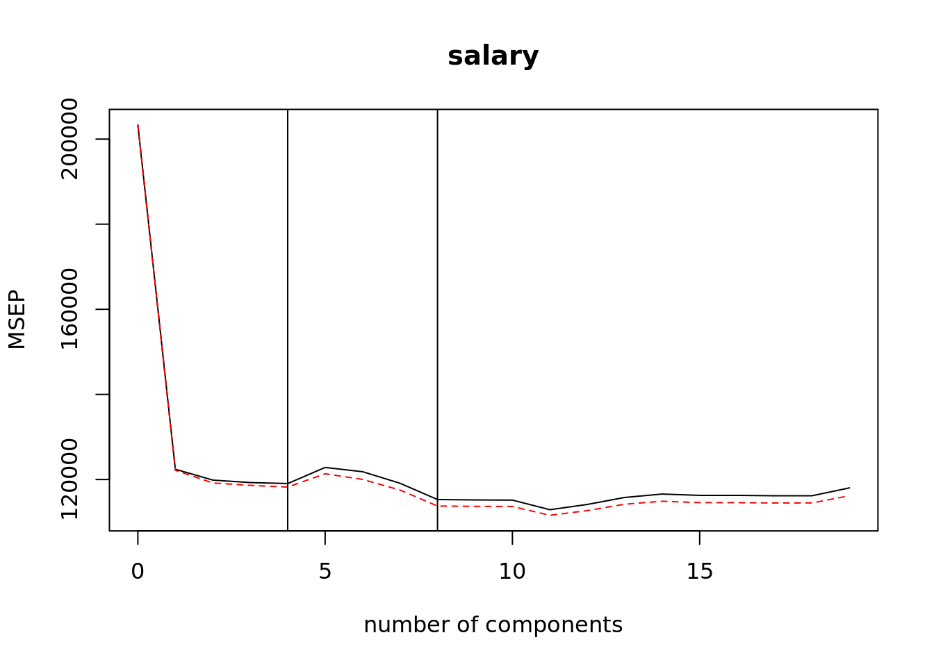
There doesn’t appear to be much difference between using 2, 3, or 4 partial least squares directions either (see plot above and table below). The fewer directions, the better because the purpose of partial least squares regression is to reduce the dimension of our predictor space. Let’s also plan on proposing a candidate model with 2 parial leat squares directions.
pls_cv %>%
  summary()
## Data: X dimension: 224 19
## Y dimension: 224 1
## Fit method: kernelpls
## Number of components considered: 19
##
## VALIDATION: RMSEP
## Cross-validated using 10 random segments.
## (Intercept) 1 comps 2 comps 3 comps 4 comps 5 comps 6 comps 7 comps 8 comps 9 comps
## CV 450.9 349.9 346.2 345.4 345.0 350.5 349.0 345.1 339.5 339.4
## adjCV 450.9 349.5 345.2 344.4 343.8 348.4 346.4 342.8 337.3 337.2
## 10 comps 11 comps 12 comps 13 comps 14 comps 15 comps 16 comps 17 comps 18 comps
## CV 339.3 336 337.9 340.3 341.4 341.0 341.0 340.8 340.9
## adjCV 337.1 334 335.7 337.9 339.0 338.5 338.5 338.3 338.4
## 19 comps
## CV 343.6
## adjCV 340.9
##
## TRAINING: % variance explained
## 1 comps 2 comps 3 comps 4 comps 5 comps 6 comps 7 comps 8 comps 9 comps 10 comps
## X 38.48 48.29 64.29 73.60 79.24 84.54 88.19 90.19 93.13 95.72
## salary 42.08 47.15 48.54 49.83 52.00 53.79 54.68 55.73 56.04 56.21
## 11 comps 12 comps 13 comps 14 comps 15 comps 16 comps 17 comps 18 comps 19 comps
## X 96.94 97.73 98.36 98.67 99.02 99.23 99.66 99.99 100.0
## salary 56.45 56.58 56.66 56.78 56.85 56.88 56.89 56.90 56.9Now that we have identified the best \(m\) for each method we need to fit them to the entire model building dataset hitter_mod_bldg_dat. These will be the candidate models produced by principal component regression and partial least squares regression. We do this within a tibble framework so that later we are able to calculate each model’s test error (test mse) on hitter_mod_comp_dat. This will allow us to easily compare all of our candidate models against each other in order to pick a final prediction model.
hitter_dim_reduct <- tibble(
  train = hitter_mod_bldg_dat %>% list(),
  test  = hitter_mod_comp_dat %>% list()
  ) %>%
  mutate(
    pcr_7m = map(train, ~ pcr(salary ~ . -name, data = .x, ncomp = 7)),
    pls_8m = map(train, ~ plsr(salary ~ . -name, data = .x, ncomp = 8)),
    pls_4m = map(train, ~ plsr(salary ~ . -name, data = .x, ncomp = 4)),
    pls_2m = map(train, ~ plsr(salary ~ . -name, data = .x, ncomp = 2))
    ) %>%
  pivot_longer(cols = c(-test, -train), names_to = "method", values_to = "fit")
6.5 Final Model Selection
We will need to calculate the test error for each candidate model produced by the several methods we have previously fit.
# Test error for regsubset fits
regsubset_error <- hitter_regsubsets %>%
  mutate(test_mse = map2(fit, test, ~ test_mse_regsubset(.x, salary ~ . -name, .y))) %>%
  unnest(test_mse) %>%
  group_by(method) %>%
  filter(model_index == max(model_index)) %>%
  select(method, test_mse) %>%
  ungroup()

# Test error for ridge and lasso fits
glmnet_error <- hitter_glmnet %>%
  mutate(pred = map2(fit, test, predict),
         test_mse = map2_dbl(test, pred, ~ mean((.x$salary - .y)^2))) %>%
  unnest(test_mse) %>%
  select(method, test_mse)

# Test error for pcr and plsr fits
dim_reduce_error <- hitter_dim_reduct %>%
  mutate(pred = pmap(list(fit, test, c(7, 8, 4, 2)), predict),
         test_mse = map2_dbl(test, pred, ~ mean((.x$salary - .y)^2))) %>%
  unnest(test_mse)  %>%
  select(method, test_mse)

# Test errors ccombined and organzied
regsubset_error %>%
  bind_rows(glmnet_error) %>%
  bind_rows(dim_reduce_error) %>%
  arrange(test_mse) %>%
knitr::kable(digits = 2)| method | test_mse |
|---|---|
| pls_4m | 112607.6 |
| pcr_7m | 114341.1 |
| ridge_min | 131184.2 |
| lasso_min | 133106.5 |
| lasso_1se | 134645.3 |
| pls_8m | 135032.4 |
| fwd_selection_5 | 136732.3 |
| fwd_selection_6 | 136732.3 |
| back_selection | 136732.3 |
| best_subset | 136732.3 |
| ridge_1se | 140772.4 |
| pls_2m | 143780.4 |
Appears that the model build using PLS with 4 partial least squares directions is the best (lowest test mse). Though PCR with 7 components isn’t too far behind. If we are hoping to have a model that we might be able to more easily interpret then the model with 8 predictors selected by both backwards and best subset selection would be useful.