1 Simple Linear Regression

Read section 3.1 of the book before using these notes.

Note that in this course, lecture notes are not sufficient, you must read the book for better understanding. Lecture notes are just implementing the concepts of the book on a dataset, but not explaining the concepts elaborately.

1.1 Simple Linear Regression

import pandas as pd
import numpy as np
import statsmodels.formula.api as smf
import statsmodels.api as sm
import seaborn as sns
import matplotlib.pyplot as plt
from matplotlib.patches import Patch
from matplotlib.lines import Line2D
from sklearn.linear_model import LinearRegression
from sklearn.metrics import mean_squared_error, mean_absolute_error, r2_score

Develop a simple linear regression model that predicts car price based on engine size. Datasets to be used: Car_features_train.csv, Car_prices_train.csv

# We are reading training data ONLY at this point.
# Test data is already separated in another file
trainf = pd.read_csv('./Datasets/Car_features_train.csv') # Predictors
trainp = pd.read_csv('./Datasets/Car_prices_train.csv') # Response
train = pd.merge(trainf,trainp)
train.head()

	carID	brand	model	year	transmission	mileage	fuelType	tax	mpg	engineSize	price
0	18473	bmw	6 Series	2020	Semi-Auto	11	Diesel	145	53.3282	3.0	37980
1	15064	bmw	6 Series	2019	Semi-Auto	10813	Diesel	145	53.0430	3.0	33980
2	18268	bmw	6 Series	2020	Semi-Auto	6	Diesel	145	53.4379	3.0	36850
3	18480	bmw	6 Series	2017	Semi-Auto	18895	Diesel	145	51.5140	3.0	25998
4	18492	bmw	6 Series	2015	Automatic	62953	Diesel	160	51.4903	3.0	18990

1.1.1 Training with `statsmodels`

Here, we will use the statsmodels.formula.api module of the statsmodels library. The use of “API” here doesn’t refer to a traditional external web API but rather an interface within the library for users to interact with and perform specific tasks. The statsmodels.formula.api module provides a formulaic interface to the statsmodels library. A formula is a compact way to specify statistical models using a formula language. This module allows users to define statistical models using formulas similar to those used in R.

So, in summary, the statsmodels.formula.api module provides a formulaic interface as part of the statsmodels library, allowing users to specify statistical models using a convenient and concise formula syntax.

# Let's create the model
    
# ols stands for Ordinary Least Squares - the name of the algorithm that optimizes Linear Regression models

# data input needs the dataframe that has the predictor and the response
# formula input needs to:
    # be a string
    # have the following syntax: "response~predictor"
    
# Using engineSize to predict price
ols_object = smf.ols(formula = 'price~engineSize', data = train)

#Using the fit() function of the 'ols' class to fit the model, i.e., train the model
model = ols_object.fit()

#Printing model summary which contains among other things, the model coefficients
model.summary()

OLS Regression Results
Dep. Variable:	price	R-squared:	0.390
Model:	OLS	Adj. R-squared:	0.390
Method:	Least Squares	F-statistic:	3177.
Date:	Tue, 16 Jan 2024	Prob (F-statistic):	0.00
Time:	16:46:33	Log-Likelihood:	-53949.
No. Observations:	4960	AIC:	1.079e+05
Df Residuals:	4958	BIC:	1.079e+05
Df Model:	1
Covariance Type:	nonrobust

	coef	std err	t	P>\|t\|	[0.025	0.975]
Intercept	-4122.0357	522.260	-7.893	0.000	-5145.896	-3098.176
engineSize	1.299e+04	230.450	56.361	0.000	1.25e+04	1.34e+04

Omnibus:	1271.986	Durbin-Watson:	0.517
Prob(Omnibus):	0.000	Jarque-Bera (JB):	6490.719
Skew:	1.137	Prob(JB):	0.00
Kurtosis:	8.122	Cond. No.	7.64

Notes:
[1] Standard Errors assume that the covariance matrix of the errors is correctly specified.

The model equation is: $\hat{price}$ = -4122.0357 + 12990 * engineSize

R-squared is 39%. This is the proportion of variance in car price explained by engineSize.
The coef of engineSize ($\hat{\beta}_1$) is statistically significant ($p$-value = 0). There is a linear relationship between X and Y.
The 95% CI of $\hat{\beta}_1$ is [1.25e+04, 1.34e+04].
PI is not shown here.

The coefficient of engineSize is 1.299e+04. - Unit change in engineSize increases the expected price by $\$$ 12,990. - An increase of 3 increases the price by $\$$ (3*1.299e+04) = $\$$ 38,970.

The coefficients can also be returned directly usign the params attribute of the model object returned by the fit() method of the ols class:

model.params

Intercept     -4122.035744
engineSize    12988.281021
dtype: float64

Visualize the regression line

sns.set(font_scale=1.25)
ax = sns.scatterplot(x = train.engineSize, y = train.price,color = 'orange')
sns.lineplot(x = train.engineSize, y = model.fittedvalues,color = 'blue')
plt.xlim(-1,7)
plt.xlabel('Engine size (in litres)')
plt.ylabel('Car price')
legend_elements = [Line2D([0], [0], color='blue', lw=4, label='Predicted (Model)'),
                   Line2D([0], [0], marker='o', color='w', label='Actual',
                          markerfacecolor='orange', markersize=10)]
ax.legend(handles=legend_elements, loc='upper left');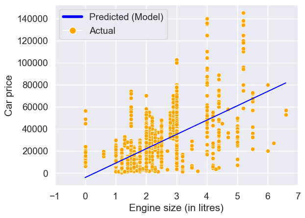

Note that the above plot can be made directly using the seaborn function regplot(). The function regplot() fits a simple linear regression model with y as the response, and x as the predictor, and then plots the model over a scatteplot of the data.

ax = sns.regplot(x = 'engineSize', y = 'price', data = train, color = 'orange',line_kws={"color": "blue"})
plt.xlim(-1,7)
plt.xlabel('Engine size (in litres)')
plt.ylabel('Car price')
ax.yaxis.set_major_formatter('${x:,.0f}')
ax.legend(handles=legend_elements, loc='upper left');
#Note that some of the engineSize values are 0. They are incorrect, and should ideally be imputed before developing the model.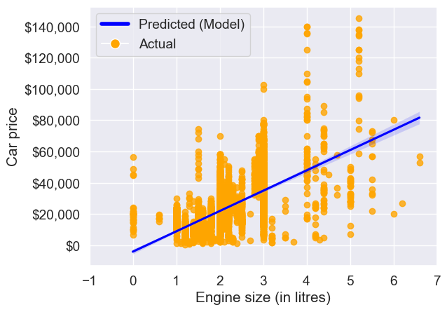

The light shaded region around the blue line in the above plot is the confidence interval.

Predict the car price for the cars in the test dataset. Datasets to be used: Car_features_test.csv, Car_prices_test.csv

Now that the model has been trained, let us evaluate it on unseen data. Make sure that the columns names of the predictors are the same in train and test datasets.

# Read the test data
testf = pd.read_csv('./Datasets/Car_features_test.csv') # Predictors
testp = pd.read_csv('./Datasets/Car_prices_test.csv') # Response
test = pd.merge(testf, testp)

#Using the predict() function associated with the 'model' object to make predictions of car price on test (unknown) data
pred_price = model.predict(testf)#Note that the predict() function finds the predictor 'engineSize' in the testf dataframe, and plugs its values in the regression equation for prediction.

Make a visualization that compares the predicted car prices with the actual car prices

sns.scatterplot(x = testp.price, y = pred_price, color = 'orange')
#In case of a perfect prediction, all the points must lie on the line x = y.
ax = sns.lineplot(x = [0,testp.price.max()], y = [0,testp.price.max()],color='blue') #Plotting the line x = y.
plt.xlabel('Actual price')
plt.ylabel('Predicted price')
ax.yaxis.set_major_formatter('${x:,.0f}')
ax.xaxis.set_major_formatter('${x:,.0f}')
plt.xticks(rotation=20);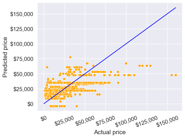

The prediction doesn’t look too good. This is because we are just using one predictor - engine size. We can probably improve the model by adding more predictors when we learn multiple linear regression.

What is the RMSE of the predicted car price on unseen data?

np.sqrt(((testp.price - pred_price)**2).mean())

12995.106451548696

The root mean squared error in predicting car price is around $13k.

What is the residual standard error based on the training data?

np.sqrt(model.mse_resid)

12810.109175214138

The residual standard error on the training data is close to the RMSE on the test data. This shows that the performance of the model on unknown data is comparable to its performance on known data. This implies that the model is not overfitting, which is good! In case we overfit a model on the training data, its performance on unknown data is likely to be worse than that on the training data.

Find the confidence and prediction intervals of the predicted car price

#Using the get_prediction() function associated with the 'model' object to get the intervals
intervals = model.get_prediction(testf)

#The function requires specifying alpha (probability of Type 1 error) instead of the confidence level to get the intervals
intervals.summary_frame(alpha=0.05)

	mean	mean_se	mean_ci_lower	mean_ci_upper	obs_ci_lower	obs_ci_upper
0	34842.807319	271.666459	34310.220826	35375.393812	9723.677232	59961.937406
1	34842.807319	271.666459	34310.220826	35375.393812	9723.677232	59961.937406
2	34842.807319	271.666459	34310.220826	35375.393812	9723.677232	59961.937406
3	8866.245277	316.580850	8245.606701	9486.883853	-16254.905974	33987.396528
4	47831.088340	468.949360	46911.740050	48750.436631	22700.782946	72961.393735
...	...	...	...	...	...	...
2667	47831.088340	468.949360	46911.740050	48750.436631	22700.782946	72961.393735
2668	34842.807319	271.666459	34310.220826	35375.393812	9723.677232	59961.937406
2669	8866.245277	316.580850	8245.606701	9486.883853	-16254.905974	33987.396528
2670	21854.526298	184.135754	21493.538727	22215.513869	-3261.551421	46970.604017
2671	21854.526298	184.135754	21493.538727	22215.513869	-3261.551421	46970.604017

2672 rows × 6 columns

Show the regression line predicting car price based on engine size for test data. Also show the confidence and prediction intervals for the car price.

interval_table = intervals.summary_frame(alpha=0.05)

ax = sns.scatterplot(x = testf.engineSize, y = pred_price,color = 'orange', s = 10)
sns.lineplot(x = testf.engineSize, y = pred_price, color = 'red')
sns.lineplot(x = testf.engineSize, y = interval_table.mean_ci_lower, color = 'blue')
sns.lineplot(x = testf.engineSize, y = interval_table.mean_ci_upper, color = 'blue')
sns.lineplot(x = testf.engineSize, y = interval_table.obs_ci_lower, color = 'green')
sns.lineplot(x = testf.engineSize, y = interval_table.obs_ci_upper, color = 'green')

legend_elements = [Line2D([0], [0], color='red', label='Mean prediction'),
                   Line2D([0], [0], color='blue', label='Confidence interval'),
                  Line2D([0], [0], color='green', label='Prediction interval')]
ax.legend(handles=legend_elements, loc='upper left')
plt.xlabel('Engine size (in litres)')
plt.ylabel('Car price')
ax.yaxis.set_major_formatter('${x:,.0f}');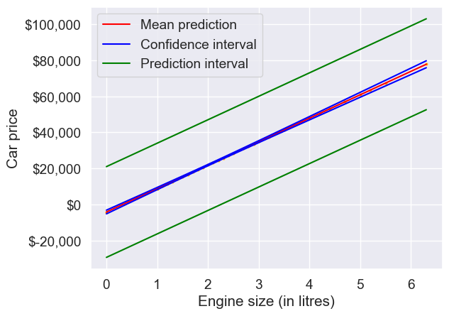

1.1.2 Training with `sklearn`

# Create the model as an object

model = LinearRegression() # No inputs, this will change for other models

# Train the model - separate the predictor(s) and the response for this!
X_train = train[['engineSize']]
y_train = train[['price']]

# Note that both are dfs, NOT series - necessary to avoid errors

model.fit(X_train, y_train)

# Check the slight syntax differences
    # predictors and response separate
    # We need to manually slice the predictor column(s) we want to include
    # No need to assign to an output
    
# Return the parameters
print("Coefficient of engine size = ", model.coef_) # slope
print("Intercept = ", model.intercept_) # intercept

# No .summary() here! - impossible to do much inference; this is a shortcoming of sklearn

Coefficient of engine size =  [[12988.28102112]]
Intercept =  [-4122.03574424]

# Prediction

# Again, separate the predictor(s) and the response of interest
X_test = test[['engineSize']]
y_test = test[['price']].to_numpy() # Easier to handle with calculations as np array

y_pred = model.predict(X_test)

# Evaluate
model_rmse = np.sqrt(np.mean((y_pred - y_test)**2)) # RMSE
model_mae = np.mean(np.abs(y_pred - y_test)) # MAE

print('Test RMSE: ', model_rmse)

Test RMSE:  12995.106451548696

# Easier way to calculate metrics with sklearn tools

# Note that we have imported the functions 'mean_squared_error' and 'mean_absolute_error'
# from the sklearn.metrics module (check top of the code)

model_rmse = np.sqrt(mean_squared_error(y_test,y_pred))
model_mae = mean_absolute_error(y_test,y_pred)
print('Test RMSE: ', model_rmse)
print('Test MAE: ', model_mae)

Test RMSE:  12995.106451548696
Test MAE:  9411.325912951994

y_pred_train = model.predict(X_train)
print('Train R-squared:', r2_score(y_train, y_pred_train))
print('Test R-squared:', r2_score(y_test, y_pred))

Train R-squared: 0.39049842625794573
Test R-squared: 0.3869900378620146

Note: Why did we repeat the same task in two different libraries?

statsmodels and sklearn have different advantages - we will use both for our purposes
- statsmodels returns a lot of statistical output, which is very helpful for inference (coming up next) but it has a limited variety of models.
- With statsmodels, you may have columns in your DataFrame in addition to predictors and response, while with sklearn you need to make separate objects consisting of only the predictors and the response.
- sklearn includes many models (Lasso and Ridge this quarter, many others next quarter) and helpful tools/functions (like metrics) that statsmodels does not but it does not have any inference tools.

1.1.3 Training with `statsmodels.api`

Earlier we had used the statsmodels.formula.api module, where we had to put the regression model as a formula. We can also use the statsmodels.api module to develop a regression model. The syntax of training a model with the OLS() function in this module is similar to that of sklearn’s LinearRegression() function. However, the order in which the predictors and response are specified is different. The formula-style syntax of the statsmodels.formula.api module is generally preferred. However, depending on the situation, the OLS() syntax of statsmodels.api may be preferred.

Note that you will manually need to add the predictor (a column of ones) corresponding to the intercept to train the model with this method.

# Create the model as an object

# Train the model - separate the predictor(s) and the response for this!
X_train = train[['engineSize']]
y_train = train[['price']]

X_train_with_intercept = np.concatenate((np.ones(X_train.shape[0]).reshape(-1,1), X_train), axis = 1)

model = sm.OLS(y_train, X_train_with_intercept).fit()
    
# Return the parameters
print(model.params)

const    -4122.035744
x1       12988.281021
dtype: float64

The model summary and all other attributes and methods of the model object are the same as that with the object created using the statsmodels.formula.api module.

model.summary()

OLS Regression Results
Dep. Variable:	price	R-squared:	0.390
Model:	OLS	Adj. R-squared:	0.390
Method:	Least Squares	F-statistic:	3177.
Date:	Mon, 08 Jan 2024	Prob (F-statistic):	0.00
Time:	11:17:55	Log-Likelihood:	-53949.
No. Observations:	4960	AIC:	1.079e+05
Df Residuals:	4958	BIC:	1.079e+05
Df Model:	1
Covariance Type:	nonrobust

	coef	std err	t	P>\|t\|	[0.025	0.975]
const	-4122.0357	522.260	-7.893	0.000	-5145.896	-3098.176
x1	1.299e+04	230.450	56.361	0.000	1.25e+04	1.34e+04

Omnibus:	1271.986	Durbin-Watson:	0.517
Prob(Omnibus):	0.000	Jarque-Bera (JB):	6490.719
Skew:	1.137	Prob(JB):	0.00
Kurtosis:	8.122	Cond. No.	7.64

Notes:
[1] Standard Errors assume that the covariance matrix of the errors is correctly specified.

1.1 Simple Linear Regression

1.1.1 Training with statsmodels

1.1.2 Training with sklearn

1.1.3 Training with statsmodels.api

1.1.1 Training with `statsmodels`

1.1.2 Training with `sklearn`

1.1.3 Training with `statsmodels.api`