%pylab inline
import pandas as pd
import seaborn as sns
import statsmodels.api as sm
plt.rcParams['figure.figsize'] = [9, 5]
Populating the interactive namespace from numpy and matplotlibRead section 3.3.3 (2) of the book before using these notes.
Note that in this course, lecture notes are not sufficient, you must read the book for better understanding. Lecture notes are just implementing the concepts of the book on a dataset, but not explaining the concepts elaborately.
Below is an example showing violation of the autocorrelation assumption (refer to the book to understand autocorrelation) in linear regression. Subsequently, it is shown that addressing the assumption violation leads to a much better model fit.
Example: Using linear regression models to predict electricity demand in Toronto, CA.
We have hourly power demand and temperature (in Celsius) data from 2017 to 2020.
We are going to build a linear model to predict the hourly power demand for the next day (for example, when it is 1/1/2021, we predict hourly demand on 1/2/2021 using historical data and the weather forecasts).
When we are building a model, it is important to keep in mind what data we can use as features. For this model:
We cannot use previous hourly data as features. (Although in a high frequency setting, it is possible)
The temperature in our raw data can not be used directly, since it is the actual, not the forecasted temperature. We are going to use the previous day temperature as the forecast.
Source: Keep it simple, keep it linear: A linear regression model for time series
%pylab inline
import pandas as pd
import seaborn as sns
import statsmodels.api as sm
plt.rcParams['figure.figsize'] = [9, 5]Populating the interactive namespace from numpy and matplotlib# A few helper functions
import numpy.ma as ma
from scipy.stats.stats import pearsonr, normaltest
from scipy.spatial.distance import correlation
def build_model(features):
X=sm.add_constant(df[features])
y=df['power']
model = sm.OLS(y,X, missing='drop').fit()
predictions = model.predict(X)
display(model.summary())
res=y-predictions
return res
def plt_residual(res):
plt.plot(range(len(res)), res)
plt.ylabel('Residual')
plt.xlabel("Hour")
def plt_residual_lag(res, nlag):
x=res.values
y=res.shift(nlag).values
sns.kdeplot(x,y=y,color='blue',shade=True )
plt.xlabel('res')
plt.ylabel("res-lag-{}".format(nlag))
rho,p=corrcoef(x,y)
plt.title("n_lag={} hours, correlation={:f}".format(nlag, rho))
def plt_acf(res):
plt.rcParams['figure.figsize'] = [18, 5]
acorr = sm.tsa.acf(res.dropna(), nlags = len(res.dropna())-1)
fig, (ax1, ax2) = plt.subplots(1, 2)
ax1.plot(acorr)
ax1.set_ylabel('corr')
ax1.set_xlabel('n_lag')
ax1.set_title('Auto Correlation')
ax2.plot(acorr[:4*7*24])
ax2.set_ylabel('corr')
ax2.set_xlabel('n_lag')
ax2.set_title('Auto Correlation (4-week zoomed in) ')
plt.show()
pd.set_option('display.max_columns', None)
adf=pd.DataFrame(np.round(acorr[:30*24],2).reshape([30, 24] ))
adf.index.name='day'
display(adf)
plt.rcParams['figure.figsize'] = [9, 5]
def corrcoef(x,y):
a,b=ma.masked_invalid(x),ma.masked_invalid(y)
msk = (~a.mask & ~b.mask)
return pearsonr(x[msk],y[msk])[0], normaltest(res, nan_policy='omit')[1]df=pd.read_csv("./Datasets/Toronto_power_demand.csv", parse_dates=['Date'], index_col=0)
df['temperature']=df['temperature'].shift(24*1)
df.tail()| Date | Hour | power | temperature | |
|---|---|---|---|---|
| key | ||||
| 20201231:19 | 2020-12-31 | 19 | 5948 | 4.9 |
| 20201231:20 | 2020-12-31 | 20 | 5741 | 4.5 |
| 20201231:21 | 2020-12-31 | 21 | 5527 | 3.7 |
| 20201231:22 | 2020-12-31 | 22 | 5301 | 2.9 |
| 20201231:23 | 2020-12-31 | 23 | 5094 | 2.1 |
ndays=len(set(df['Date']))
print("There are {} rows, which is {}*24={}, for {} days. And The data is already in sorted order" .format(df.shape[0], ndays, ndays*24, ndays))
There are 35064 rows, which is 1461*24=35064, for 1461 days. And The data is already in sorted orderprint("It is natural to think that there is a relationship between power demand and temperature.")
sns.kdeplot(df['temperature'].values, y=df['power'].values,color='blue',shade=True )
plt.title("Power Demand vs Temperature")It is natural to think that there is a relationship between power demand and temperature.Text(0.5, 1.0, 'Power Demand vs Temperature')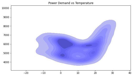
print("""
It is not a linear relationship. We create two features corresponding to hot and cold weather, which makes \
it possible to develop a linear model.
""")
is_hot=(df['temperature']>15).astype(int)
print("{:f}% of data points are hot".format(is_hot.mean()*100))
df['temp_hot']=df['temperature']*is_hot
df['temp_cold']=df['temperature']*(1-is_hot)
df.tail()
It is not a linear relationship. We create two features corresponding to hot and cold weather, which makes it possible to develop a linear model.

34.813484% of data points are hot| Date | Hour | power | temperature | temp_hot | temp_cold | |
|---|---|---|---|---|---|---|
| key | ||||||
| 20201231:19 | 2020-12-31 | 19 | 5948 | 4.9 | 0.0 | 4.9 |
| 20201231:20 | 2020-12-31 | 20 | 5741 | 4.5 | 0.0 | 4.5 |
| 20201231:21 | 2020-12-31 | 21 | 5527 | 3.7 | 0.0 | 3.7 |
| 20201231:22 | 2020-12-31 | 22 | 5301 | 2.9 | 0.0 | 2.9 |
| 20201231:23 | 2020-12-31 | 23 | 5094 | 2.1 | 0.0 | 2.1 |
res=build_model(['temp_hot', 'temp_cold'])| Dep. Variable: | power | R-squared: | 0.195 |
|---|---|---|---|
| Model: | OLS | Adj. R-squared: | 0.195 |
| Method: | Least Squares | F-statistic: | 4251. |
| Date: | Sun, 05 Feb 2023 | Prob (F-statistic): | 0.00 |
| Time: | 23:15:53 | Log-Likelihood: | -2.8766e+05 |
| No. Observations: | 35040 | AIC: | 5.753e+05 |
| Df Residuals: | 35037 | BIC: | 5.753e+05 |
| Df Model: | 2 | ||
| Covariance Type: | nonrobust |
| coef | std err | t | P>|t| | [0.025 | 0.975] | |
|---|---|---|---|---|---|---|
| const | 5501.3027 | 6.222 | 884.115 | 0.000 | 5489.107 | 5513.499 |
| temp_hot | 31.8488 | 0.462 | 68.911 | 0.000 | 30.943 | 32.755 |
| temp_cold | -37.5088 | 0.827 | -45.364 | 0.000 | -39.129 | -35.888 |
| Omnibus: | 945.032 | Durbin-Watson: | 0.093 |
|---|---|---|---|
| Prob(Omnibus): | 0.000 | Jarque-Bera (JB): | 469.200 |
| Skew: | 0.034 | Prob(JB): | 1.30e-102 |
| Kurtosis: | 2.437 | Cond. No. | 17.0 |
plt_residual(res) 
print("acf shows that there is a strong correlation for 24 lags, which is one day.")
plt_acf(res)
acf shows that there is a strong correlation for 24 lags, which is one day.C:\Users\akl0407\Anaconda3\lib\site-packages\statsmodels\tsa\stattools.py:667: FutureWarning: fft=True will become the default after the release of the 0.12 release of statsmodels. To suppress this warning, explicitly set fft=False.
warnings.warn(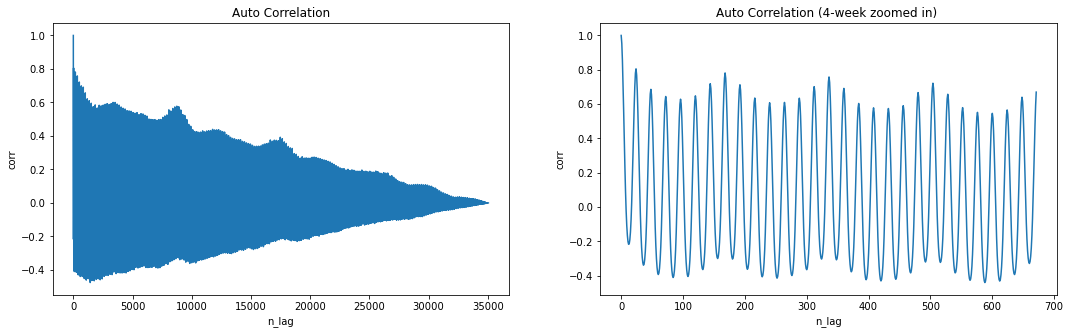
| 0 | 1 | 2 | 3 | 4 | 5 | 6 | 7 | 8 | 9 | 10 | 11 | 12 | 13 | 14 | 15 | 16 | 17 | 18 | 19 | 20 | 21 | 22 | 23 | |
|---|---|---|---|---|---|---|---|---|---|---|---|---|---|---|---|---|---|---|---|---|---|---|---|---|
| day | ||||||||||||||||||||||||
| 0 | 1.00 | 0.95 | 0.85 | 0.72 | 0.56 | 0.40 | 0.24 | 0.09 | -0.02 | -0.11 | -0.16 | -0.20 | -0.22 | -0.21 | -0.19 | -0.14 | -0.07 | 0.03 | 0.15 | 0.30 | 0.45 | 0.58 | 0.70 | 0.78 |
| 1 | 0.81 | 0.77 | 0.68 | 0.55 | 0.40 | 0.25 | 0.09 | -0.04 | -0.15 | -0.23 | -0.29 | -0.32 | -0.34 | -0.33 | -0.31 | -0.26 | -0.19 | -0.09 | 0.04 | 0.18 | 0.33 | 0.47 | 0.58 | 0.66 |
| 2 | 0.69 | 0.65 | 0.57 | 0.45 | 0.31 | 0.16 | 0.01 | -0.12 | -0.22 | -0.30 | -0.35 | -0.38 | -0.39 | -0.38 | -0.36 | -0.31 | -0.23 | -0.13 | -0.00 | 0.14 | 0.29 | 0.42 | 0.54 | 0.62 |
| 3 | 0.64 | 0.61 | 0.53 | 0.42 | 0.28 | 0.13 | -0.01 | -0.14 | -0.24 | -0.32 | -0.37 | -0.40 | -0.41 | -0.40 | -0.37 | -0.32 | -0.25 | -0.15 | -0.02 | 0.12 | 0.27 | 0.41 | 0.52 | 0.60 |
| 4 | 0.63 | 0.60 | 0.52 | 0.41 | 0.27 | 0.12 | -0.02 | -0.14 | -0.24 | -0.32 | -0.37 | -0.40 | -0.40 | -0.39 | -0.36 | -0.31 | -0.24 | -0.13 | -0.01 | 0.14 | 0.28 | 0.42 | 0.54 | 0.62 |
| 5 | 0.65 | 0.62 | 0.54 | 0.43 | 0.30 | 0.15 | 0.01 | -0.11 | -0.21 | -0.28 | -0.33 | -0.36 | -0.36 | -0.35 | -0.32 | -0.27 | -0.19 | -0.08 | 0.04 | 0.19 | 0.34 | 0.48 | 0.60 | 0.69 |
| 6 | 0.72 | 0.69 | 0.61 | 0.50 | 0.36 | 0.21 | 0.07 | -0.05 | -0.15 | -0.22 | -0.27 | -0.29 | -0.30 | -0.29 | -0.26 | -0.21 | -0.13 | -0.02 | 0.11 | 0.25 | 0.40 | 0.55 | 0.67 | 0.75 |
| 7 | 0.78 | 0.75 | 0.67 | 0.54 | 0.40 | 0.25 | 0.10 | -0.03 | -0.13 | -0.21 | -0.26 | -0.29 | -0.30 | -0.30 | -0.27 | -0.22 | -0.15 | -0.05 | 0.07 | 0.21 | 0.36 | 0.49 | 0.61 | 0.69 |
| 8 | 0.71 | 0.68 | 0.60 | 0.48 | 0.34 | 0.19 | 0.04 | -0.09 | -0.19 | -0.27 | -0.32 | -0.35 | -0.36 | -0.36 | -0.33 | -0.28 | -0.21 | -0.12 | 0.01 | 0.14 | 0.29 | 0.42 | 0.53 | 0.61 |
| 9 | 0.64 | 0.61 | 0.53 | 0.41 | 0.27 | 0.13 | -0.02 | -0.14 | -0.24 | -0.32 | -0.37 | -0.40 | -0.41 | -0.40 | -0.37 | -0.32 | -0.25 | -0.15 | -0.03 | 0.11 | 0.26 | 0.39 | 0.50 | 0.58 |
| 10 | 0.61 | 0.58 | 0.50 | 0.39 | 0.25 | 0.11 | -0.03 | -0.16 | -0.26 | -0.33 | -0.38 | -0.40 | -0.41 | -0.40 | -0.38 | -0.33 | -0.25 | -0.15 | -0.03 | 0.11 | 0.26 | 0.39 | 0.50 | 0.58 |
| 11 | 0.61 | 0.58 | 0.51 | 0.39 | 0.26 | 0.12 | -0.02 | -0.14 | -0.24 | -0.32 | -0.36 | -0.39 | -0.40 | -0.39 | -0.36 | -0.31 | -0.24 | -0.14 | -0.01 | 0.13 | 0.28 | 0.41 | 0.53 | 0.61 |
| 12 | 0.63 | 0.61 | 0.53 | 0.42 | 0.28 | 0.14 | 0.00 | -0.12 | -0.22 | -0.29 | -0.33 | -0.36 | -0.36 | -0.35 | -0.32 | -0.27 | -0.19 | -0.09 | 0.04 | 0.18 | 0.33 | 0.47 | 0.59 | 0.67 |
| 13 | 0.70 | 0.67 | 0.60 | 0.48 | 0.35 | 0.20 | 0.06 | -0.06 | -0.16 | -0.23 | -0.27 | -0.30 | -0.30 | -0.29 | -0.26 | -0.21 | -0.14 | -0.03 | 0.09 | 0.24 | 0.39 | 0.53 | 0.65 | 0.73 |
| 14 | 0.76 | 0.73 | 0.64 | 0.52 | 0.38 | 0.23 | 0.09 | -0.04 | -0.14 | -0.22 | -0.27 | -0.30 | -0.31 | -0.30 | -0.27 | -0.23 | -0.16 | -0.06 | 0.06 | 0.20 | 0.34 | 0.48 | 0.59 | 0.66 |
| 15 | 0.69 | 0.66 | 0.58 | 0.46 | 0.32 | 0.17 | 0.03 | -0.10 | -0.20 | -0.28 | -0.33 | -0.36 | -0.38 | -0.37 | -0.35 | -0.30 | -0.23 | -0.14 | -0.02 | 0.12 | 0.26 | 0.39 | 0.50 | 0.58 |
| 16 | 0.60 | 0.57 | 0.50 | 0.38 | 0.25 | 0.10 | -0.04 | -0.16 | -0.26 | -0.34 | -0.38 | -0.41 | -0.42 | -0.41 | -0.39 | -0.34 | -0.27 | -0.17 | -0.05 | 0.09 | 0.23 | 0.36 | 0.48 | 0.55 |
| 17 | 0.58 | 0.55 | 0.47 | 0.36 | 0.23 | 0.09 | -0.05 | -0.17 | -0.27 | -0.34 | -0.39 | -0.42 | -0.43 | -0.42 | -0.39 | -0.35 | -0.27 | -0.18 | -0.05 | 0.08 | 0.23 | 0.36 | 0.47 | 0.55 |
| 18 | 0.57 | 0.55 | 0.47 | 0.36 | 0.23 | 0.09 | -0.05 | -0.17 | -0.27 | -0.34 | -0.39 | -0.41 | -0.42 | -0.41 | -0.38 | -0.34 | -0.26 | -0.17 | -0.04 | 0.10 | 0.24 | 0.37 | 0.48 | 0.56 |
| 19 | 0.59 | 0.57 | 0.49 | 0.38 | 0.25 | 0.11 | -0.03 | -0.14 | -0.24 | -0.31 | -0.35 | -0.38 | -0.38 | -0.37 | -0.34 | -0.29 | -0.22 | -0.11 | 0.01 | 0.15 | 0.30 | 0.44 | 0.55 | 0.64 |
| 20 | 0.67 | 0.64 | 0.56 | 0.45 | 0.32 | 0.18 | 0.04 | -0.08 | -0.17 | -0.24 | -0.29 | -0.31 | -0.32 | -0.31 | -0.28 | -0.23 | -0.16 | -0.06 | 0.07 | 0.21 | 0.36 | 0.49 | 0.61 | 0.69 |
| 21 | 0.72 | 0.69 | 0.61 | 0.49 | 0.36 | 0.21 | 0.07 | -0.06 | -0.16 | -0.23 | -0.28 | -0.31 | -0.32 | -0.32 | -0.29 | -0.25 | -0.18 | -0.08 | 0.03 | 0.17 | 0.31 | 0.44 | 0.56 | 0.63 |
| 22 | 0.66 | 0.63 | 0.55 | 0.43 | 0.29 | 0.15 | 0.01 | -0.12 | -0.22 | -0.29 | -0.34 | -0.37 | -0.38 | -0.38 | -0.35 | -0.31 | -0.24 | -0.15 | -0.03 | 0.10 | 0.24 | 0.37 | 0.48 | 0.55 |
| 23 | 0.58 | 0.55 | 0.47 | 0.36 | 0.23 | 0.09 | -0.05 | -0.17 | -0.27 | -0.34 | -0.39 | -0.42 | -0.43 | -0.42 | -0.39 | -0.35 | -0.28 | -0.18 | -0.06 | 0.07 | 0.21 | 0.34 | 0.45 | 0.53 |
| 24 | 0.55 | 0.52 | 0.45 | 0.34 | 0.21 | 0.07 | -0.07 | -0.19 | -0.29 | -0.36 | -0.40 | -0.43 | -0.44 | -0.43 | -0.40 | -0.36 | -0.29 | -0.19 | -0.07 | 0.06 | 0.20 | 0.33 | 0.44 | 0.52 |
| 25 | 0.55 | 0.52 | 0.45 | 0.34 | 0.21 | 0.07 | -0.07 | -0.19 | -0.28 | -0.35 | -0.40 | -0.42 | -0.43 | -0.42 | -0.39 | -0.35 | -0.28 | -0.18 | -0.06 | 0.08 | 0.22 | 0.35 | 0.46 | 0.54 |
| 26 | 0.57 | 0.54 | 0.47 | 0.36 | 0.23 | 0.09 | -0.04 | -0.16 | -0.25 | -0.32 | -0.36 | -0.39 | -0.39 | -0.38 | -0.35 | -0.30 | -0.23 | -0.13 | -0.00 | 0.13 | 0.28 | 0.42 | 0.53 | 0.61 |
| 27 | 0.64 | 0.61 | 0.54 | 0.43 | 0.30 | 0.16 | 0.03 | -0.09 | -0.19 | -0.25 | -0.30 | -0.32 | -0.33 | -0.32 | -0.29 | -0.24 | -0.17 | -0.07 | 0.06 | 0.19 | 0.34 | 0.48 | 0.59 | 0.67 |
| 28 | 0.70 | 0.67 | 0.59 | 0.47 | 0.34 | 0.19 | 0.05 | -0.07 | -0.17 | -0.24 | -0.29 | -0.32 | -0.33 | -0.33 | -0.30 | -0.26 | -0.19 | -0.10 | 0.02 | 0.15 | 0.29 | 0.42 | 0.53 | 0.61 |
| 29 | 0.63 | 0.60 | 0.53 | 0.41 | 0.28 | 0.13 | -0.01 | -0.13 | -0.23 | -0.30 | -0.35 | -0.38 | -0.39 | -0.39 | -0.37 | -0.32 | -0.26 | -0.16 | -0.05 | 0.08 | 0.22 | 0.35 | 0.46 | 0.53 |
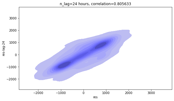
print("Although 1 hour lag correlation is more strong, but we cannot use it, as we intend to predict \
the power consumption for the next day.")
plt_residual_lag(res,1)
plt.show()
plt_residual_lag(res,24)
Although 1 hour lag correlation is more strong, but we cannot use it, as we intend to predict the power consumption for the next day.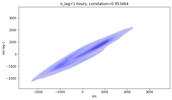
df['power_lag_1_day']=df['power'].shift(24)
df.tail()| key | Date | Hour | power | temperature | temp_hot | temp_cold | power_lag_1_day | |
|---|---|---|---|---|---|---|---|---|
| 35059 | 20201231:19 | 2020-12-31 | 19 | 5948 | 4.9 | 0.0 | 4.9 | 6163.0 |
| 35060 | 20201231:20 | 2020-12-31 | 20 | 5741 | 4.5 | 0.0 | 4.5 | 5983.0 |
| 35061 | 20201231:21 | 2020-12-31 | 21 | 5527 | 3.7 | 0.0 | 3.7 | 5727.0 |
| 35062 | 20201231:22 | 2020-12-31 | 22 | 5301 | 2.9 | 0.0 | 2.9 | 5428.0 |
| 35063 | 20201231:23 | 2020-12-31 | 23 | 5094 | 2.1 | 0.0 | 2.1 | 5104.0 |
res=build_model(['temp_hot', 'temp_cold', 'power_lag_1_day' ])/usr/local/lib/python3.8/dist-packages/statsmodels/tsa/tsatools.py:142: FutureWarning: In a future version of pandas all arguments of concat except for the argument 'objs' will be keyword-only
x = pd.concat(x[::order], 1)| Dep. Variable: | power | R-squared: | 0.794 |
|---|---|---|---|
| Model: | OLS | Adj. R-squared: | 0.794 |
| Method: | Least Squares | F-statistic: | 4.513e+04 |
| Date: | Sun, 22 Jan 2023 | Prob (F-statistic): | 0.00 |
| Time: | 19:21:14 | Log-Likelihood: | -2.6375e+05 |
| No. Observations: | 35040 | AIC: | 5.275e+05 |
| Df Residuals: | 35036 | BIC: | 5.275e+05 |
| Df Model: | 3 | ||
| Covariance Type: | nonrobust |
| coef | std err | t | P>|t| | [0.025 | 0.975] | |
|---|---|---|---|---|---|---|
| const | 689.2701 | 15.384 | 44.806 | 0.000 | 659.118 | 719.422 |
| temp_hot | 3.2158 | 0.250 | 12.853 | 0.000 | 2.725 | 3.706 |
| temp_cold | -1.3464 | 0.433 | -3.110 | 0.002 | -2.195 | -0.498 |
| power_lag_1_day | 0.8747 | 0.003 | 319.552 | 0.000 | 0.869 | 0.880 |
| Omnibus: | 2035.537 | Durbin-Watson: | 0.041 |
|---|---|---|---|
| Prob(Omnibus): | 0.000 | Jarque-Bera (JB): | 5794.290 |
| Skew: | 0.301 | Prob(JB): | 0.00 |
| Kurtosis: | 4.899 | Cond. No. | 3.69e+04 |
plt_residual(res)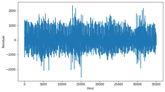
plt_acf(res)/usr/local/lib/python3.8/dist-packages/statsmodels/tsa/stattools.py:667: FutureWarning: fft=True will become the default after the release of the 0.12 release of statsmodels. To suppress this warning, explicitly set fft=False.
warnings.warn(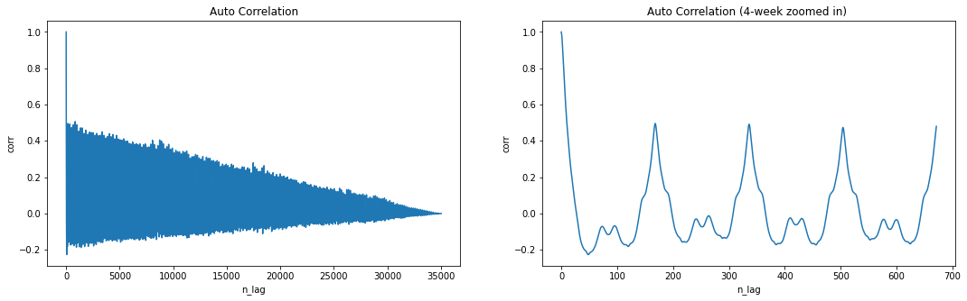
| 0 | 1 | 2 | 3 | 4 | 5 | 6 | 7 | 8 | 9 | 10 | 11 | 12 | 13 | 14 | 15 | 16 | 17 | 18 | 19 | 20 | 21 | 22 | 23 | |
|---|---|---|---|---|---|---|---|---|---|---|---|---|---|---|---|---|---|---|---|---|---|---|---|---|
| day | ||||||||||||||||||||||||
| 0 | 1.00 | 0.98 | 0.93 | 0.87 | 0.81 | 0.75 | 0.70 | 0.64 | 0.59 | 0.54 | 0.50 | 0.46 | 0.42 | 0.39 | 0.35 | 0.31 | 0.28 | 0.25 | 0.22 | 0.20 | 0.17 | 0.15 | 0.12 | 0.09 |
| 1 | 0.07 | 0.05 | 0.03 | 0.00 | -0.02 | -0.04 | -0.06 | -0.08 | -0.10 | -0.12 | -0.14 | -0.15 | -0.16 | -0.17 | -0.18 | -0.19 | -0.19 | -0.20 | -0.20 | -0.20 | -0.21 | -0.21 | -0.22 | -0.22 |
| 2 | -0.23 | -0.23 | -0.22 | -0.22 | -0.21 | -0.21 | -0.21 | -0.21 | -0.21 | -0.20 | -0.20 | -0.19 | -0.18 | -0.18 | -0.17 | -0.16 | -0.15 | -0.14 | -0.12 | -0.11 | -0.10 | -0.09 | -0.08 | -0.08 |
| 3 | -0.07 | -0.07 | -0.07 | -0.07 | -0.08 | -0.09 | -0.09 | -0.10 | -0.11 | -0.11 | -0.11 | -0.12 | -0.12 | -0.12 | -0.11 | -0.11 | -0.11 | -0.10 | -0.09 | -0.09 | -0.08 | -0.07 | -0.07 | -0.07 |
| 4 | -0.07 | -0.07 | -0.07 | -0.08 | -0.09 | -0.10 | -0.11 | -0.12 | -0.13 | -0.14 | -0.14 | -0.15 | -0.16 | -0.16 | -0.16 | -0.17 | -0.17 | -0.17 | -0.17 | -0.17 | -0.17 | -0.17 | -0.18 | -0.18 |
| 5 | -0.18 | -0.18 | -0.17 | -0.17 | -0.17 | -0.16 | -0.16 | -0.16 | -0.16 | -0.15 | -0.14 | -0.14 | -0.13 | -0.12 | -0.10 | -0.09 | -0.07 | -0.05 | -0.04 | -0.02 | 0.00 | 0.02 | 0.04 | 0.06 |
| 6 | 0.07 | 0.08 | 0.09 | 0.09 | 0.10 | 0.10 | 0.11 | 0.12 | 0.13 | 0.14 | 0.16 | 0.18 | 0.19 | 0.21 | 0.23 | 0.25 | 0.27 | 0.30 | 0.33 | 0.36 | 0.39 | 0.43 | 0.46 | 0.48 |
| 7 | 0.50 | 0.49 | 0.46 | 0.43 | 0.40 | 0.37 | 0.34 | 0.31 | 0.28 | 0.26 | 0.24 | 0.22 | 0.21 | 0.19 | 0.18 | 0.16 | 0.15 | 0.14 | 0.13 | 0.13 | 0.12 | 0.12 | 0.12 | 0.11 |
| 8 | 0.10 | 0.09 | 0.07 | 0.06 | 0.04 | 0.02 | -0.00 | -0.02 | -0.04 | -0.05 | -0.07 | -0.08 | -0.09 | -0.10 | -0.11 | -0.11 | -0.12 | -0.12 | -0.13 | -0.13 | -0.13 | -0.14 | -0.15 | -0.15 |
| 9 | -0.16 | -0.16 | -0.16 | -0.15 | -0.16 | -0.16 | -0.16 | -0.16 | -0.16 | -0.16 | -0.15 | -0.15 | -0.14 | -0.14 | -0.13 | -0.12 | -0.11 | -0.10 | -0.09 | -0.07 | -0.06 | -0.05 | -0.04 | -0.04 |
| 10 | -0.03 | -0.03 | -0.03 | -0.03 | -0.04 | -0.04 | -0.05 | -0.06 | -0.06 | -0.07 | -0.07 | -0.07 | -0.07 | -0.07 | -0.07 | -0.07 | -0.06 | -0.05 | -0.05 | -0.04 | -0.03 | -0.02 | -0.02 | -0.01 |
| 11 | -0.01 | -0.01 | -0.02 | -0.03 | -0.03 | -0.04 | -0.05 | -0.06 | -0.07 | -0.08 | -0.09 | -0.10 | -0.11 | -0.11 | -0.11 | -0.12 | -0.12 | -0.12 | -0.12 | -0.12 | -0.12 | -0.12 | -0.13 | -0.13 |
| 12 | -0.14 | -0.14 | -0.13 | -0.13 | -0.13 | -0.13 | -0.14 | -0.14 | -0.13 | -0.13 | -0.13 | -0.12 | -0.11 | -0.10 | -0.09 | -0.08 | -0.06 | -0.05 | -0.03 | -0.01 | 0.01 | 0.03 | 0.05 | 0.07 |
| 13 | 0.08 | 0.09 | 0.10 | 0.10 | 0.11 | 0.11 | 0.12 | 0.13 | 0.14 | 0.15 | 0.17 | 0.18 | 0.20 | 0.22 | 0.23 | 0.26 | 0.28 | 0.31 | 0.33 | 0.36 | 0.40 | 0.43 | 0.46 | 0.48 |
| 14 | 0.49 | 0.48 | 0.46 | 0.43 | 0.40 | 0.37 | 0.34 | 0.31 | 0.28 | 0.26 | 0.24 | 0.23 | 0.21 | 0.20 | 0.18 | 0.17 | 0.15 | 0.14 | 0.13 | 0.13 | 0.12 | 0.12 | 0.12 | 0.11 |
| 15 | 0.10 | 0.09 | 0.07 | 0.05 | 0.03 | 0.01 | -0.01 | -0.03 | -0.05 | -0.07 | -0.08 | -0.10 | -0.11 | -0.12 | -0.13 | -0.14 | -0.14 | -0.15 | -0.15 | -0.15 | -0.15 | -0.16 | -0.16 | -0.17 |
| 16 | -0.17 | -0.17 | -0.17 | -0.17 | -0.16 | -0.16 | -0.17 | -0.17 | -0.16 | -0.16 | -0.16 | -0.16 | -0.15 | -0.14 | -0.13 | -0.12 | -0.11 | -0.10 | -0.09 | -0.07 | -0.06 | -0.05 | -0.04 | -0.03 |
| 17 | -0.03 | -0.02 | -0.02 | -0.03 | -0.03 | -0.04 | -0.04 | -0.05 | -0.05 | -0.06 | -0.06 | -0.06 | -0.06 | -0.06 | -0.06 | -0.06 | -0.05 | -0.05 | -0.04 | -0.04 | -0.03 | -0.03 | -0.03 | -0.03 |
| 18 | -0.03 | -0.04 | -0.04 | -0.05 | -0.06 | -0.08 | -0.09 | -0.10 | -0.11 | -0.12 | -0.13 | -0.14 | -0.15 | -0.15 | -0.16 | -0.16 | -0.16 | -0.17 | -0.17 | -0.17 | -0.17 | -0.17 | -0.17 | -0.17 |
| 19 | -0.17 | -0.17 | -0.16 | -0.16 | -0.15 | -0.15 | -0.15 | -0.15 | -0.14 | -0.13 | -0.13 | -0.12 | -0.11 | -0.10 | -0.09 | -0.07 | -0.05 | -0.03 | -0.02 | 0.00 | 0.03 | 0.05 | 0.07 | 0.08 |
| 20 | 0.10 | 0.10 | 0.11 | 0.11 | 0.12 | 0.12 | 0.12 | 0.13 | 0.14 | 0.15 | 0.17 | 0.18 | 0.20 | 0.21 | 0.23 | 0.25 | 0.27 | 0.29 | 0.32 | 0.35 | 0.38 | 0.41 | 0.44 | 0.47 |
| 21 | 0.47 | 0.46 | 0.44 | 0.41 | 0.38 | 0.35 | 0.32 | 0.29 | 0.26 | 0.24 | 0.22 | 0.21 | 0.19 | 0.18 | 0.16 | 0.15 | 0.13 | 0.13 | 0.12 | 0.12 | 0.11 | 0.11 | 0.11 | 0.10 |
| 22 | 0.10 | 0.09 | 0.07 | 0.05 | 0.03 | 0.01 | -0.00 | -0.02 | -0.04 | -0.05 | -0.07 | -0.08 | -0.09 | -0.10 | -0.10 | -0.11 | -0.12 | -0.12 | -0.12 | -0.13 | -0.13 | -0.13 | -0.14 | -0.14 |
| 23 | -0.14 | -0.14 | -0.14 | -0.14 | -0.14 | -0.14 | -0.14 | -0.14 | -0.14 | -0.14 | -0.13 | -0.13 | -0.13 | -0.12 | -0.11 | -0.11 | -0.10 | -0.09 | -0.08 | -0.07 | -0.06 | -0.05 | -0.04 | -0.03 |
| 24 | -0.03 | -0.03 | -0.03 | -0.04 | -0.05 | -0.05 | -0.06 | -0.07 | -0.08 | -0.08 | -0.09 | -0.09 | -0.09 | -0.09 | -0.08 | -0.08 | -0.08 | -0.07 | -0.06 | -0.05 | -0.05 | -0.04 | -0.04 | -0.03 |
| 25 | -0.03 | -0.04 | -0.04 | -0.05 | -0.06 | -0.07 | -0.08 | -0.09 | -0.10 | -0.11 | -0.12 | -0.13 | -0.14 | -0.14 | -0.15 | -0.15 | -0.15 | -0.15 | -0.16 | -0.16 | -0.16 | -0.16 | -0.16 | -0.16 |
| 26 | -0.17 | -0.17 | -0.16 | -0.16 | -0.16 | -0.15 | -0.15 | -0.15 | -0.15 | -0.14 | -0.13 | -0.13 | -0.12 | -0.11 | -0.10 | -0.08 | -0.07 | -0.05 | -0.03 | -0.01 | 0.01 | 0.03 | 0.05 | 0.07 |
| 27 | 0.08 | 0.09 | 0.10 | 0.11 | 0.11 | 0.12 | 0.12 | 0.13 | 0.14 | 0.16 | 0.18 | 0.19 | 0.21 | 0.22 | 0.24 | 0.26 | 0.28 | 0.31 | 0.34 | 0.37 | 0.40 | 0.43 | 0.46 | 0.48 |
| 28 | 0.49 | 0.48 | 0.45 | 0.42 | 0.39 | 0.36 | 0.33 | 0.30 | 0.27 | 0.25 | 0.23 | 0.22 | 0.20 | 0.19 | 0.17 | 0.16 | 0.14 | 0.13 | 0.12 | 0.12 | 0.11 | 0.11 | 0.11 | 0.10 |
| 29 | 0.09 | 0.08 | 0.06 | 0.04 | 0.02 | -0.00 | -0.02 | -0.04 | -0.06 | -0.08 | -0.09 | -0.10 | -0.12 | -0.13 | -0.14 | -0.14 | -0.15 | -0.15 | -0.16 | -0.16 | -0.16 | -0.17 | -0.17 | -0.18 |
plt_residual_lag(res, 1)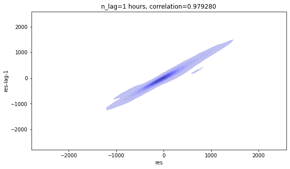
plt_residual_lag(res, 24)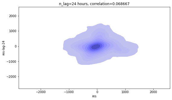
plt_residual_lag(res, 24*7)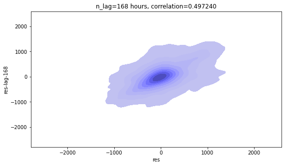
df['power_lag_1_week']=df['power'].shift(24*7)
df.tail()| key | Date | Hour | power | temperature | temp_hot | temp_cold | power_lag_1_day | power_lag_1_week | |
|---|---|---|---|---|---|---|---|---|---|
| 35059 | 20201231:19 | 2020-12-31 | 19 | 5948 | 4.9 | 0.0 | 4.9 | 6163.0 | 5833.0 |
| 35060 | 20201231:20 | 2020-12-31 | 20 | 5741 | 4.5 | 0.0 | 4.5 | 5983.0 | 5665.0 |
| 35061 | 20201231:21 | 2020-12-31 | 21 | 5527 | 3.7 | 0.0 | 3.7 | 5727.0 | 5474.0 |
| 35062 | 20201231:22 | 2020-12-31 | 22 | 5301 | 2.9 | 0.0 | 2.9 | 5428.0 | 5273.0 |
| 35063 | 20201231:23 | 2020-12-31 | 23 | 5094 | 2.1 | 0.0 | 2.1 | 5104.0 | 5010.0 |
res=build_model(['temp_hot', 'temp_cold', 'power_lag_1_day', 'power_lag_1_week' ])/usr/local/lib/python3.8/dist-packages/statsmodels/tsa/tsatools.py:142: FutureWarning: In a future version of pandas all arguments of concat except for the argument 'objs' will be keyword-only
x = pd.concat(x[::order], 1)| Dep. Variable: | power | R-squared: | 0.840 |
|---|---|---|---|
| Model: | OLS | Adj. R-squared: | 0.840 |
| Method: | Least Squares | F-statistic: | 4.585e+04 |
| Date: | Sun, 22 Jan 2023 | Prob (F-statistic): | 0.00 |
| Time: | 19:22:49 | Log-Likelihood: | -2.5830e+05 |
| No. Observations: | 34896 | AIC: | 5.166e+05 |
| Df Residuals: | 34891 | BIC: | 5.167e+05 |
| Df Model: | 4 | ||
| Covariance Type: | nonrobust |
| coef | std err | t | P>|t| | [0.025 | 0.975] | |
|---|---|---|---|---|---|---|
| const | 290.4344 | 14.166 | 20.502 | 0.000 | 262.668 | 318.201 |
| temp_hot | 3.2967 | 0.221 | 14.896 | 0.000 | 2.863 | 3.730 |
| temp_cold | -4.5938 | 0.385 | -11.943 | 0.000 | -5.348 | -3.840 |
| power_lag_1_day | 0.6114 | 0.004 | 170.709 | 0.000 | 0.604 | 0.618 |
| power_lag_1_week | 0.3342 | 0.003 | 99.595 | 0.000 | 0.328 | 0.341 |
| Omnibus: | 2729.372 | Durbin-Watson: | 0.037 |
|---|---|---|---|
| Prob(Omnibus): | 0.000 | Jarque-Bera (JB): | 11234.560 |
| Skew: | 0.299 | Prob(JB): | 0.00 |
| Kurtosis: | 5.715 | Cond. No. | 5.43e+04 |
plt_residual(res)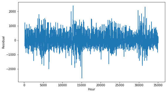
plt_acf(res)/usr/local/lib/python3.8/dist-packages/statsmodels/tsa/stattools.py:667: FutureWarning: fft=True will become the default after the release of the 0.12 release of statsmodels. To suppress this warning, explicitly set fft=False.
warnings.warn(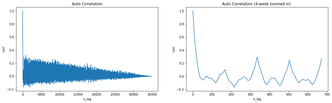
| 0 | 1 | 2 | 3 | 4 | 5 | 6 | 7 | 8 | 9 | 10 | 11 | 12 | 13 | 14 | 15 | 16 | 17 | 18 | 19 | 20 | 21 | 22 | 23 | |
|---|---|---|---|---|---|---|---|---|---|---|---|---|---|---|---|---|---|---|---|---|---|---|---|---|
| day | ||||||||||||||||||||||||
| 0 | 1.00 | 0.98 | 0.94 | 0.89 | 0.84 | 0.79 | 0.74 | 0.70 | 0.65 | 0.61 | 0.58 | 0.54 | 0.51 | 0.48 | 0.45 | 0.42 | 0.39 | 0.37 | 0.34 | 0.32 | 0.30 | 0.27 | 0.25 | 0.22 |
| 1 | 0.20 | 0.18 | 0.16 | 0.14 | 0.12 | 0.10 | 0.09 | 0.07 | 0.06 | 0.04 | 0.03 | 0.02 | 0.01 | 0.00 | -0.00 | -0.01 | -0.02 | -0.02 | -0.02 | -0.03 | -0.03 | -0.04 | -0.04 | -0.05 |
| 2 | -0.05 | -0.06 | -0.06 | -0.05 | -0.05 | -0.05 | -0.05 | -0.05 | -0.05 | -0.05 | -0.05 | -0.04 | -0.04 | -0.04 | -0.03 | -0.03 | -0.02 | -0.02 | -0.01 | -0.01 | -0.00 | -0.00 | 0.00 | 0.00 |
| 3 | 0.00 | 0.00 | 0.00 | -0.00 | -0.00 | -0.01 | -0.01 | -0.01 | -0.02 | -0.02 | -0.02 | -0.03 | -0.03 | -0.03 | -0.03 | -0.03 | -0.03 | -0.03 | -0.03 | -0.03 | -0.02 | -0.02 | -0.02 | -0.03 |
| 4 | -0.03 | -0.03 | -0.03 | -0.03 | -0.03 | -0.04 | -0.04 | -0.04 | -0.05 | -0.05 | -0.05 | -0.06 | -0.06 | -0.06 | -0.07 | -0.07 | -0.07 | -0.08 | -0.08 | -0.08 | -0.08 | -0.09 | -0.09 | -0.10 |
| 5 | -0.10 | -0.09 | -0.09 | -0.08 | -0.08 | -0.07 | -0.07 | -0.07 | -0.06 | -0.06 | -0.05 | -0.05 | -0.04 | -0.04 | -0.03 | -0.02 | -0.02 | -0.01 | -0.00 | 0.00 | 0.01 | 0.02 | 0.03 | 0.03 |
| 6 | 0.03 | 0.03 | 0.03 | 0.03 | 0.03 | 0.03 | 0.03 | 0.03 | 0.03 | 0.04 | 0.04 | 0.05 | 0.05 | 0.05 | 0.06 | 0.06 | 0.06 | 0.07 | 0.07 | 0.08 | 0.08 | 0.09 | 0.09 | 0.10 |
| 7 | 0.10 | 0.10 | 0.09 | 0.08 | 0.06 | 0.05 | 0.05 | 0.04 | 0.03 | 0.02 | 0.01 | 0.01 | 0.00 | -0.01 | -0.02 | -0.03 | -0.03 | -0.04 | -0.05 | -0.06 | -0.06 | -0.07 | -0.07 | -0.07 |
| 8 | -0.08 | -0.08 | -0.08 | -0.09 | -0.09 | -0.09 | -0.09 | -0.10 | -0.10 | -0.10 | -0.10 | -0.11 | -0.11 | -0.11 | -0.12 | -0.12 | -0.13 | -0.13 | -0.13 | -0.14 | -0.15 | -0.15 | -0.16 | -0.16 |
| 9 | -0.17 | -0.16 | -0.16 | -0.15 | -0.15 | -0.14 | -0.14 | -0.13 | -0.13 | -0.12 | -0.12 | -0.11 | -0.11 | -0.10 | -0.10 | -0.09 | -0.09 | -0.08 | -0.08 | -0.08 | -0.07 | -0.07 | -0.06 | -0.06 |
| 10 | -0.06 | -0.05 | -0.05 | -0.05 | -0.05 | -0.05 | -0.04 | -0.04 | -0.04 | -0.04 | -0.04 | -0.04 | -0.04 | -0.04 | -0.04 | -0.03 | -0.03 | -0.03 | -0.03 | -0.02 | -0.02 | -0.02 | -0.01 | -0.01 |
| 11 | -0.01 | -0.01 | -0.01 | -0.01 | -0.01 | -0.01 | -0.01 | -0.01 | -0.01 | -0.02 | -0.02 | -0.02 | -0.03 | -0.03 | -0.03 | -0.03 | -0.03 | -0.04 | -0.04 | -0.04 | -0.05 | -0.05 | -0.06 | -0.06 |
| 12 | -0.07 | -0.07 | -0.06 | -0.06 | -0.06 | -0.06 | -0.06 | -0.05 | -0.05 | -0.05 | -0.05 | -0.04 | -0.04 | -0.03 | -0.03 | -0.02 | -0.01 | -0.01 | 0.00 | 0.01 | 0.02 | 0.03 | 0.04 | 0.04 |
| 13 | 0.05 | 0.06 | 0.06 | 0.07 | 0.08 | 0.08 | 0.09 | 0.10 | 0.11 | 0.12 | 0.13 | 0.14 | 0.15 | 0.16 | 0.17 | 0.18 | 0.19 | 0.20 | 0.22 | 0.23 | 0.25 | 0.26 | 0.28 | 0.29 |
| 14 | 0.29 | 0.29 | 0.27 | 0.26 | 0.24 | 0.23 | 0.21 | 0.20 | 0.19 | 0.18 | 0.17 | 0.16 | 0.15 | 0.14 | 0.13 | 0.12 | 0.11 | 0.10 | 0.09 | 0.08 | 0.07 | 0.07 | 0.06 | 0.06 |
| 15 | 0.05 | 0.04 | 0.03 | 0.02 | 0.01 | -0.00 | -0.01 | -0.02 | -0.03 | -0.04 | -0.05 | -0.06 | -0.06 | -0.07 | -0.08 | -0.08 | -0.09 | -0.10 | -0.10 | -0.11 | -0.11 | -0.11 | -0.12 | -0.12 |
| 16 | -0.13 | -0.13 | -0.12 | -0.12 | -0.11 | -0.11 | -0.11 | -0.10 | -0.10 | -0.10 | -0.10 | -0.09 | -0.09 | -0.08 | -0.08 | -0.07 | -0.07 | -0.06 | -0.06 | -0.05 | -0.05 | -0.04 | -0.04 | -0.04 |
| 17 | -0.03 | -0.03 | -0.03 | -0.03 | -0.03 | -0.03 | -0.03 | -0.03 | -0.03 | -0.03 | -0.03 | -0.03 | -0.03 | -0.03 | -0.03 | -0.03 | -0.03 | -0.03 | -0.03 | -0.03 | -0.03 | -0.04 | -0.04 | -0.04 |
| 18 | -0.05 | -0.05 | -0.06 | -0.06 | -0.06 | -0.07 | -0.07 | -0.08 | -0.08 | -0.09 | -0.09 | -0.10 | -0.10 | -0.10 | -0.11 | -0.11 | -0.12 | -0.12 | -0.12 | -0.13 | -0.13 | -0.14 | -0.14 | -0.14 |
| 19 | -0.14 | -0.14 | -0.13 | -0.13 | -0.12 | -0.11 | -0.11 | -0.10 | -0.10 | -0.09 | -0.08 | -0.08 | -0.07 | -0.06 | -0.06 | -0.05 | -0.04 | -0.03 | -0.02 | -0.01 | -0.00 | 0.01 | 0.01 | 0.02 |
| 20 | 0.03 | 0.03 | 0.04 | 0.04 | 0.05 | 0.05 | 0.06 | 0.07 | 0.07 | 0.08 | 0.09 | 0.10 | 0.11 | 0.12 | 0.13 | 0.14 | 0.15 | 0.16 | 0.17 | 0.19 | 0.20 | 0.22 | 0.23 | 0.24 |
| 21 | 0.25 | 0.24 | 0.23 | 0.22 | 0.20 | 0.19 | 0.17 | 0.16 | 0.14 | 0.13 | 0.12 | 0.11 | 0.11 | 0.10 | 0.09 | 0.08 | 0.07 | 0.06 | 0.06 | 0.05 | 0.05 | 0.04 | 0.04 | 0.04 |
| 22 | 0.04 | 0.03 | 0.02 | 0.02 | 0.01 | 0.00 | -0.01 | -0.01 | -0.02 | -0.03 | -0.03 | -0.04 | -0.04 | -0.05 | -0.05 | -0.05 | -0.06 | -0.06 | -0.07 | -0.07 | -0.08 | -0.08 | -0.09 | -0.09 |
| 23 | -0.10 | -0.10 | -0.09 | -0.09 | -0.09 | -0.08 | -0.08 | -0.08 | -0.07 | -0.07 | -0.07 | -0.07 | -0.07 | -0.06 | -0.06 | -0.06 | -0.06 | -0.05 | -0.05 | -0.05 | -0.05 | -0.05 | -0.05 | -0.05 |
| 24 | -0.05 | -0.05 | -0.05 | -0.05 | -0.05 | -0.05 | -0.06 | -0.06 | -0.06 | -0.06 | -0.06 | -0.06 | -0.06 | -0.06 | -0.06 | -0.06 | -0.06 | -0.06 | -0.06 | -0.05 | -0.05 | -0.05 | -0.05 | -0.05 |
| 25 | -0.05 | -0.05 | -0.05 | -0.05 | -0.05 | -0.06 | -0.06 | -0.06 | -0.07 | -0.07 | -0.08 | -0.08 | -0.09 | -0.09 | -0.09 | -0.09 | -0.10 | -0.10 | -0.10 | -0.11 | -0.11 | -0.12 | -0.12 | -0.13 |
| 26 | -0.13 | -0.13 | -0.12 | -0.12 | -0.11 | -0.11 | -0.10 | -0.10 | -0.09 | -0.09 | -0.08 | -0.08 | -0.07 | -0.07 | -0.06 | -0.06 | -0.05 | -0.04 | -0.03 | -0.02 | -0.02 | -0.01 | 0.00 | 0.01 |
| 27 | 0.02 | 0.03 | 0.03 | 0.04 | 0.05 | 0.06 | 0.06 | 0.07 | 0.08 | 0.10 | 0.11 | 0.12 | 0.13 | 0.14 | 0.15 | 0.16 | 0.17 | 0.18 | 0.20 | 0.21 | 0.23 | 0.24 | 0.25 | 0.27 |
| 28 | 0.27 | 0.27 | 0.25 | 0.24 | 0.22 | 0.21 | 0.19 | 0.18 | 0.17 | 0.15 | 0.14 | 0.14 | 0.13 | 0.12 | 0.11 | 0.10 | 0.09 | 0.08 | 0.08 | 0.07 | 0.06 | 0.06 | 0.05 | 0.05 |
| 29 | 0.04 | 0.03 | 0.02 | 0.02 | 0.01 | -0.00 | -0.01 | -0.02 | -0.03 | -0.04 | -0.04 | -0.05 | -0.06 | -0.07 | -0.07 | -0.08 | -0.08 | -0.09 | -0.09 | -0.10 | -0.10 | -0.11 | -0.12 | -0.12 |
plt_residual_lag(res, 1)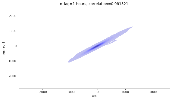
plt_residual_lag(res, 24)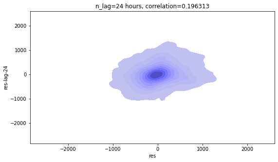
plt_residual_lag(res, 24*7)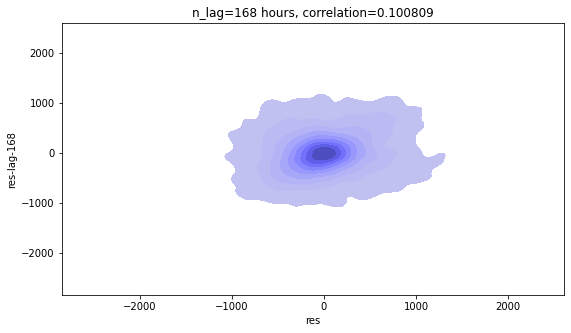
plt_residual_lag(res, 24*7*2)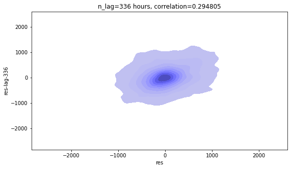
Although the data shows there is a significant (but not strong) correlation, we need to be cautious to use this feature because there are no simple reasons for this relationship.
For 1-day-lag feature, the correlation is easily understood.
For 1-week-lag feature, we could argue that the behaviour is different between weekday and weekend.
But for 2-week-lag feature, it is hard to understand especially when we have included 1-day-lag and 1-week-lag features. The relation is spurious.
df['power_lag_2_week']=df['power'].shift(24*7*2)
df.tail()| key | Date | Hour | power | temperature | temp_hot | temp_cold | power_lag_1_day | power_lag_1_week | power_lag_2_week | |
|---|---|---|---|---|---|---|---|---|---|---|
| 35059 | 20201231:19 | 2020-12-31 | 19 | 5948 | 4.9 | 0.0 | 4.9 | 6163.0 | 5833.0 | 6826.0 |
| 35060 | 20201231:20 | 2020-12-31 | 20 | 5741 | 4.5 | 0.0 | 4.5 | 5983.0 | 5665.0 | 6663.0 |
| 35061 | 20201231:21 | 2020-12-31 | 21 | 5527 | 3.7 | 0.0 | 3.7 | 5727.0 | 5474.0 | 6407.0 |
| 35062 | 20201231:22 | 2020-12-31 | 22 | 5301 | 2.9 | 0.0 | 2.9 | 5428.0 | 5273.0 | 6068.0 |
| 35063 | 20201231:23 | 2020-12-31 | 23 | 5094 | 2.1 | 0.0 | 2.1 | 5104.0 | 5010.0 | 5709.0 |
res=build_model(['temp_hot', 'temp_cold', 'power_lag_1_day','power_lag_1_week', 'power_lag_2_week' ])/usr/local/lib/python3.8/dist-packages/statsmodels/tsa/tsatools.py:142: FutureWarning: In a future version of pandas all arguments of concat except for the argument 'objs' will be keyword-only
x = pd.concat(x[::order], 1)| Dep. Variable: | power | R-squared: | 0.848 |
|---|---|---|---|
| Model: | OLS | Adj. R-squared: | 0.847 |
| Method: | Least Squares | F-statistic: | 3.860e+04 |
| Date: | Sun, 22 Jan 2023 | Prob (F-statistic): | 0.00 |
| Time: | 19:25:04 | Log-Likelihood: | -2.5626e+05 |
| No. Observations: | 34728 | AIC: | 5.125e+05 |
| Df Residuals: | 34722 | BIC: | 5.126e+05 |
| Df Model: | 5 | ||
| Covariance Type: | nonrobust |
| coef | std err | t | P>|t| | [0.025 | 0.975] | |
|---|---|---|---|---|---|---|
| const | 200.8402 | 14.046 | 14.298 | 0.000 | 173.309 | 228.371 |
| temp_hot | 3.2508 | 0.217 | 14.983 | 0.000 | 2.826 | 3.676 |
| temp_cold | -5.6865 | 0.379 | -15.005 | 0.000 | -6.429 | -4.944 |
| power_lag_1_day | 0.5637 | 0.004 | 152.597 | 0.000 | 0.556 | 0.571 |
| power_lag_1_week | 0.2415 | 0.004 | 60.139 | 0.000 | 0.234 | 0.249 |
| power_lag_2_week | 0.1565 | 0.004 | 40.465 | 0.000 | 0.149 | 0.164 |
| Omnibus: | 2229.659 | Durbin-Watson: | 0.036 |
|---|---|---|---|
| Prob(Omnibus): | 0.000 | Jarque-Bera (JB): | 7850.238 |
| Skew: | 0.262 | Prob(JB): | 0.00 |
| Kurtosis: | 5.270 | Cond. No. | 6.72e+04 |
plt_acf(res)/usr/local/lib/python3.8/dist-packages/statsmodels/tsa/stattools.py:667: FutureWarning: fft=True will become the default after the release of the 0.12 release of statsmodels. To suppress this warning, explicitly set fft=False.
warnings.warn(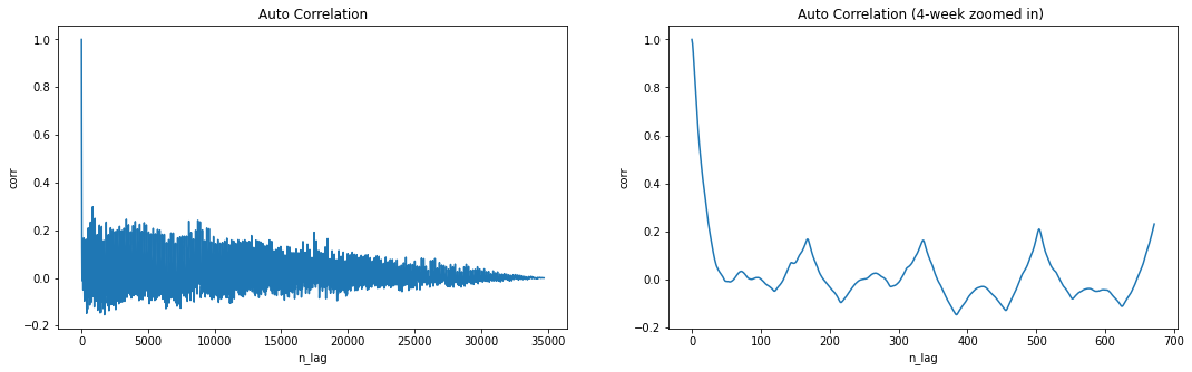
| 0 | 1 | 2 | 3 | 4 | 5 | 6 | 7 | 8 | 9 | 10 | 11 | 12 | 13 | 14 | 15 | 16 | 17 | 18 | 19 | 20 | 21 | 22 | 23 | |
|---|---|---|---|---|---|---|---|---|---|---|---|---|---|---|---|---|---|---|---|---|---|---|---|---|
| day | ||||||||||||||||||||||||
| 0 | 1.00 | 0.98 | 0.94 | 0.90 | 0.85 | 0.80 | 0.75 | 0.71 | 0.67 | 0.63 | 0.59 | 0.56 | 0.53 | 0.50 | 0.47 | 0.44 | 0.41 | 0.39 | 0.37 | 0.35 | 0.33 | 0.30 | 0.28 | 0.25 |
| 1 | 0.23 | 0.21 | 0.20 | 0.18 | 0.16 | 0.14 | 0.13 | 0.11 | 0.10 | 0.08 | 0.07 | 0.06 | 0.05 | 0.05 | 0.04 | 0.04 | 0.03 | 0.03 | 0.02 | 0.02 | 0.01 | 0.01 | 0.00 | -0.00 |
| 2 | -0.01 | -0.01 | -0.01 | -0.01 | -0.01 | -0.01 | -0.01 | -0.01 | -0.01 | -0.01 | -0.01 | -0.01 | -0.00 | -0.00 | 0.00 | 0.01 | 0.01 | 0.02 | 0.02 | 0.02 | 0.03 | 0.03 | 0.03 | 0.03 |
| 3 | 0.03 | 0.03 | 0.03 | 0.03 | 0.02 | 0.02 | 0.02 | 0.01 | 0.01 | 0.01 | 0.00 | 0.00 | 0.00 | -0.00 | -0.00 | -0.00 | 0.00 | 0.00 | 0.00 | 0.00 | 0.01 | 0.01 | 0.01 | 0.01 |
| 4 | 0.01 | 0.01 | 0.00 | 0.00 | 0.00 | -0.00 | -0.00 | -0.01 | -0.01 | -0.01 | -0.02 | -0.02 | -0.02 | -0.02 | -0.03 | -0.03 | -0.03 | -0.03 | -0.03 | -0.04 | -0.04 | -0.04 | -0.05 | -0.05 |
| 5 | -0.05 | -0.05 | -0.04 | -0.04 | -0.04 | -0.03 | -0.03 | -0.03 | -0.02 | -0.02 | -0.02 | -0.01 | -0.01 | -0.00 | 0.01 | 0.01 | 0.02 | 0.03 | 0.03 | 0.04 | 0.05 | 0.05 | 0.06 | 0.07 |
| 6 | 0.07 | 0.07 | 0.07 | 0.07 | 0.07 | 0.07 | 0.07 | 0.07 | 0.08 | 0.08 | 0.09 | 0.09 | 0.10 | 0.10 | 0.11 | 0.11 | 0.12 | 0.12 | 0.13 | 0.14 | 0.14 | 0.15 | 0.16 | 0.16 |
| 7 | 0.17 | 0.16 | 0.15 | 0.14 | 0.13 | 0.12 | 0.11 | 0.10 | 0.09 | 0.09 | 0.08 | 0.07 | 0.07 | 0.06 | 0.05 | 0.04 | 0.03 | 0.03 | 0.02 | 0.02 | 0.01 | 0.01 | 0.00 | -0.00 |
| 8 | -0.00 | -0.01 | -0.01 | -0.02 | -0.02 | -0.02 | -0.03 | -0.03 | -0.03 | -0.04 | -0.04 | -0.04 | -0.05 | -0.05 | -0.05 | -0.06 | -0.06 | -0.06 | -0.07 | -0.07 | -0.08 | -0.08 | -0.09 | -0.09 |
| 9 | -0.10 | -0.10 | -0.09 | -0.09 | -0.09 | -0.08 | -0.08 | -0.08 | -0.07 | -0.07 | -0.06 | -0.06 | -0.06 | -0.05 | -0.05 | -0.04 | -0.04 | -0.03 | -0.03 | -0.03 | -0.02 | -0.02 | -0.02 | -0.01 |
| 10 | -0.01 | -0.01 | -0.01 | -0.01 | -0.00 | -0.00 | -0.00 | -0.00 | -0.00 | -0.00 | 0.00 | 0.00 | 0.00 | 0.00 | 0.00 | 0.00 | 0.01 | 0.01 | 0.01 | 0.01 | 0.02 | 0.02 | 0.02 | 0.02 |
| 11 | 0.02 | 0.02 | 0.02 | 0.02 | 0.02 | 0.02 | 0.02 | 0.02 | 0.02 | 0.02 | 0.01 | 0.01 | 0.01 | 0.01 | 0.01 | 0.00 | 0.00 | -0.00 | -0.00 | -0.01 | -0.01 | -0.02 | -0.02 | -0.03 |
| 12 | -0.03 | -0.03 | -0.03 | -0.03 | -0.03 | -0.03 | -0.03 | -0.03 | -0.02 | -0.02 | -0.02 | -0.02 | -0.01 | -0.01 | -0.01 | -0.00 | 0.00 | 0.01 | 0.01 | 0.02 | 0.02 | 0.03 | 0.04 | 0.04 |
| 13 | 0.05 | 0.05 | 0.05 | 0.05 | 0.06 | 0.06 | 0.06 | 0.07 | 0.07 | 0.08 | 0.08 | 0.09 | 0.09 | 0.10 | 0.10 | 0.11 | 0.11 | 0.12 | 0.13 | 0.13 | 0.14 | 0.15 | 0.16 | 0.16 |
| 14 | 0.16 | 0.16 | 0.15 | 0.14 | 0.13 | 0.12 | 0.11 | 0.10 | 0.09 | 0.08 | 0.08 | 0.07 | 0.06 | 0.06 | 0.05 | 0.04 | 0.03 | 0.02 | 0.01 | 0.01 | 0.00 | -0.01 | -0.01 | -0.02 |
| 15 | -0.02 | -0.03 | -0.03 | -0.04 | -0.05 | -0.05 | -0.06 | -0.06 | -0.07 | -0.08 | -0.08 | -0.09 | -0.09 | -0.10 | -0.10 | -0.11 | -0.11 | -0.12 | -0.12 | -0.13 | -0.13 | -0.14 | -0.14 | -0.15 |
| 16 | -0.15 | -0.15 | -0.14 | -0.14 | -0.13 | -0.13 | -0.12 | -0.12 | -0.11 | -0.11 | -0.11 | -0.10 | -0.10 | -0.10 | -0.09 | -0.09 | -0.08 | -0.08 | -0.07 | -0.07 | -0.06 | -0.06 | -0.06 | -0.06 |
| 17 | -0.05 | -0.05 | -0.05 | -0.04 | -0.04 | -0.04 | -0.04 | -0.04 | -0.03 | -0.03 | -0.03 | -0.03 | -0.03 | -0.03 | -0.03 | -0.03 | -0.03 | -0.03 | -0.03 | -0.04 | -0.04 | -0.04 | -0.04 | -0.05 |
| 18 | -0.05 | -0.05 | -0.06 | -0.06 | -0.06 | -0.07 | -0.07 | -0.07 | -0.07 | -0.08 | -0.08 | -0.09 | -0.09 | -0.09 | -0.10 | -0.10 | -0.10 | -0.11 | -0.11 | -0.11 | -0.12 | -0.12 | -0.13 | -0.13 |
| 19 | -0.13 | -0.13 | -0.12 | -0.11 | -0.11 | -0.10 | -0.09 | -0.09 | -0.08 | -0.08 | -0.07 | -0.07 | -0.06 | -0.05 | -0.05 | -0.04 | -0.03 | -0.03 | -0.02 | -0.01 | -0.00 | 0.00 | 0.01 | 0.02 |
| 20 | 0.02 | 0.03 | 0.03 | 0.04 | 0.04 | 0.05 | 0.05 | 0.06 | 0.07 | 0.07 | 0.08 | 0.09 | 0.10 | 0.10 | 0.11 | 0.12 | 0.13 | 0.14 | 0.15 | 0.16 | 0.17 | 0.18 | 0.20 | 0.21 |
| 21 | 0.21 | 0.20 | 0.19 | 0.18 | 0.17 | 0.16 | 0.15 | 0.13 | 0.12 | 0.11 | 0.11 | 0.10 | 0.09 | 0.09 | 0.08 | 0.07 | 0.06 | 0.06 | 0.05 | 0.05 | 0.04 | 0.04 | 0.04 | 0.03 |
| 22 | 0.03 | 0.03 | 0.02 | 0.02 | 0.01 | 0.00 | -0.00 | -0.01 | -0.01 | -0.02 | -0.02 | -0.03 | -0.03 | -0.04 | -0.04 | -0.04 | -0.05 | -0.05 | -0.05 | -0.06 | -0.06 | -0.07 | -0.07 | -0.08 |
| 23 | -0.08 | -0.08 | -0.08 | -0.08 | -0.07 | -0.07 | -0.07 | -0.06 | -0.06 | -0.06 | -0.06 | -0.05 | -0.05 | -0.05 | -0.05 | -0.05 | -0.05 | -0.04 | -0.04 | -0.04 | -0.04 | -0.04 | -0.04 | -0.04 |
| 24 | -0.04 | -0.04 | -0.04 | -0.04 | -0.04 | -0.04 | -0.05 | -0.05 | -0.05 | -0.05 | -0.05 | -0.05 | -0.05 | -0.05 | -0.05 | -0.05 | -0.05 | -0.05 | -0.05 | -0.04 | -0.04 | -0.04 | -0.04 | -0.04 |
| 25 | -0.04 | -0.04 | -0.05 | -0.05 | -0.05 | -0.05 | -0.05 | -0.06 | -0.06 | -0.06 | -0.07 | -0.07 | -0.07 | -0.08 | -0.08 | -0.08 | -0.08 | -0.09 | -0.09 | -0.10 | -0.10 | -0.10 | -0.11 | -0.11 |
| 26 | -0.11 | -0.11 | -0.11 | -0.10 | -0.10 | -0.09 | -0.09 | -0.08 | -0.08 | -0.08 | -0.07 | -0.07 | -0.06 | -0.06 | -0.05 | -0.05 | -0.04 | -0.03 | -0.03 | -0.02 | -0.01 | -0.01 | 0.00 | 0.01 |
| 27 | 0.02 | 0.02 | 0.03 | 0.04 | 0.04 | 0.05 | 0.06 | 0.07 | 0.07 | 0.09 | 0.10 | 0.11 | 0.11 | 0.12 | 0.13 | 0.14 | 0.15 | 0.16 | 0.17 | 0.18 | 0.20 | 0.21 | 0.22 | 0.23 |
| 28 | 0.23 | 0.23 | 0.22 | 0.20 | 0.19 | 0.18 | 0.17 | 0.16 | 0.15 | 0.14 | 0.13 | 0.12 | 0.11 | 0.11 | 0.10 | 0.09 | 0.08 | 0.08 | 0.07 | 0.06 | 0.06 | 0.05 | 0.04 | 0.04 |
| 29 | 0.03 | 0.03 | 0.02 | 0.01 | 0.01 | -0.00 | -0.01 | -0.01 | -0.02 | -0.03 | -0.03 | -0.04 | -0.05 | -0.05 | -0.06 | -0.06 | -0.07 | -0.07 | -0.08 | -0.08 | -0.09 | -0.09 | -0.10 | -0.10 |
plt_residual_lag(res, 1)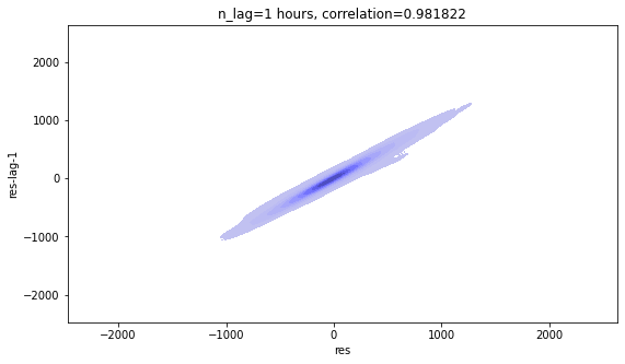
plt_residual_lag(res, 24)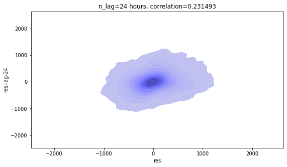
plt_residual_lag(res, 24*7)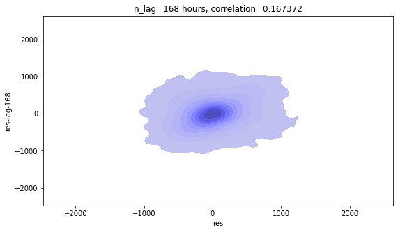
plt_residual_lag(res, 24*7*2)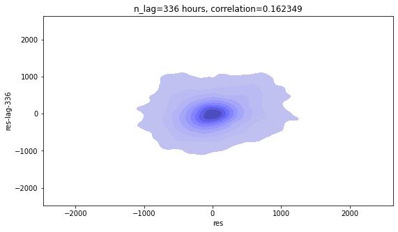
We saw that with 2-week-lag feature, the \(R^2\) only increased a little. The model summary seems still good so we could keep it. However, from the viewpoint of interpretation I may remove it.
One may also notice that the 1-day-lag correlation becomes bigger although 1-day-lag feature is already in the model. It is probably because of the multicollinearity between the lag features.
The following table shows the correlation between lag features.
df[['power_lag_1_day','power_lag_1_week', 'power_lag_2_week' ]].corr()| power_lag_1_day | power_lag_1_week | power_lag_2_week | |
|---|---|---|---|
| power_lag_1_day | 1.000000 | 0.768394 | 0.745817 |
| power_lag_1_week | 0.768394 | 1.000000 | 0.819955 |
| power_lag_2_week | 0.745817 | 0.819955 | 1.000000 |