4 Model assumptions

Read section 3.3.3 (1 & 3) of the book before using these notes.

Note that in this course, lecture notes are not sufficient, you must read the book for better understanding. Lecture notes are just implementing the concepts of the book on a dataset, but not explaining the concepts elaborately.

Consider the model with interactions and transformation developed previously.

import pandas as pd
import numpy as np
import statsmodels.formula.api as smf
import seaborn as sns
import matplotlib.pyplot as plt

trainf = pd.read_csv('./Datasets/Car_features_train.csv')
trainp = pd.read_csv('./Datasets/Car_prices_train.csv')
testf = pd.read_csv('./Datasets/Car_features_test.csv')
testp = pd.read_csv('./Datasets/Car_prices_test.csv')
train = pd.merge(trainf,trainp)
train.head()

	carID	brand	model	year	transmission	mileage	fuelType	tax	mpg	engineSize	price
0	18473	bmw	6 Series	2020	Semi-Auto	11	Diesel	145	53.3282	3.0	37980
1	15064	bmw	6 Series	2019	Semi-Auto	10813	Diesel	145	53.0430	3.0	33980
2	18268	bmw	6 Series	2020	Semi-Auto	6	Diesel	145	53.4379	3.0	36850
3	18480	bmw	6 Series	2017	Semi-Auto	18895	Diesel	145	51.5140	3.0	25998
4	18492	bmw	6 Series	2015	Automatic	62953	Diesel	160	51.4903	3.0	18990

ols_object = smf.ols(formula = 'price~(year+engineSize+mileage+mpg)**2+I(mileage**2)', data = train)
model = ols_object.fit()
model.summary()

OLS Regression Results
Dep. Variable:	price	R-squared:	0.732
Model:	OLS	Adj. R-squared:	0.731
Method:	Least Squares	F-statistic:	1229.
Date:	Wed, 25 Jan 2023	Prob (F-statistic):	0.00
Time:	11:36:00	Log-Likelihood:	-51911.
No. Observations:	4960	AIC:	1.038e+05
Df Residuals:	4948	BIC:	1.039e+05
Df Model:	11
Covariance Type:	nonrobust

	coef	std err	t	P>\|t\|	[0.025	0.975]
Intercept	-1.282e+06	7.14e+05	-1.795	0.073	-2.68e+06	1.18e+05
year	632.3954	353.865	1.787	0.074	-61.338	1326.128
engineSize	-1.465e+06	1.61e+05	-9.129	0.000	-1.78e+06	-1.15e+06
mileage	56.4581	3.811	14.815	0.000	48.987	63.929
mpg	-2.951e+04	9550.775	-3.089	0.002	-4.82e+04	-1.08e+04
year:engineSize	735.8074	79.532	9.252	0.000	579.890	891.725
year:mileage	-0.0281	0.002	-14.898	0.000	-0.032	-0.024
year:mpg	14.6915	4.731	3.105	0.002	5.417	23.966
engineSize:mileage	-0.0808	0.011	-7.143	0.000	-0.103	-0.059
engineSize:mpg	-120.5780	11.384	-10.592	0.000	-142.896	-98.260
mileage:mpg	0.0026	0.000	5.173	0.000	0.002	0.004
I(mileage ** 2)	3.495e-07	1.56e-07	2.236	0.025	4.31e-08	6.56e-07

Omnibus:	1958.631	Durbin-Watson:	0.542
Prob(Omnibus):	0.000	Jarque-Bera (JB):	44560.042
Skew:	1.349	Prob(JB):	0.00
Kurtosis:	17.434	Cond. No.	1.73e+13

Notes:
[1] Standard Errors assume that the covariance matrix of the errors is correctly specified.
[2] The condition number is large, 1.73e+13. This might indicate that there are
strong multicollinearity or other numerical problems.

np.sqrt(model.mse_resid)

8502.851955843495

#Computing RMSE on test data
pred_price = model.predict(testf)
np.sqrt(((testp.price - pred_price)**2).mean())

8708.676318160937

#Computing MAE on test data
pred_price = model.predict(testf)
(np.abs(testp.price - pred_price)).mean()

5395.006622253402

Let us check if this model satisfies the assumptions of the linear regression model

4.1 Non-linearity of data

We have assumed that there is a linear relationship between the predictors and the response. Residual plots, which are scatter plots of residuals vs fitted values, can be used to identify non-linearity. Fitted values are the values estimated by the model on training data, denoted by \(\hat y_i\), and residuals are given by \(e_i = y_i - \hat y_i\).

#Plotting residuals vs fitted values
plt.rcParams["figure.figsize"] = (9,6)
sns.set(font_scale=1.25)
ax = sns.scatterplot(x = model.fittedvalues, y=model.resid,color = 'orange')
sns.lineplot(x = [pred_price.min(),pred_price.max()],y = [0,0],color = 'blue')
plt.xlabel('Fitted values')
plt.ylabel('Residuals')
ax.yaxis.set_major_formatter('${x:,.0f}')
ax.xaxis.set_major_formatter('${x:,.0f}')

The model seems to satisfy this assumption, as we do not observe a strong pattern in the residuals around the line Residuals = 0. Residuals are distributed more or less in a similar manner on both sides of the blue line for all fitted values.

For the model to satisfy the linearity assumption perfectly, the points above the line (Residuals = 0), should be mirror image of the points below the line, i.e., the blue line in the above plot should act as a mirror.

What to do if there is non-linear association (page 94 of book): If the residual plot indicates that there are non-linear associations in the data, then a simple approach is to use non-linear transformations of the predictors, such as \(log X, \sqrt X\), and \(X^2\), in the regression model.

4.2 Non-constant variance of error terms

The variance of the error terms is assumed to be constant, i.e., \(Var(\epsilon_i) = \sigma^2\), and this assumption is used while deriving the standard errors of the regression coefficients. The standard errors in turn are used to test the significant of the predictors, and obtain their confidence interval. Thus, violation of this assumption may lead to incorrect inference. Non-constant variance of error terms, or violation of the constant variance assumption, is called heteroscedasticity.

This assumption can be checked by plotting the residuals against fitted values.

#Plotting residuals vs fitted values
ax = sns.scatterplot(x = model.fittedvalues, y=model.resid,color = 'orange')
sns.lineplot(x = [pred_price.min(),pred_price.max()],y = [0,0],color = 'blue')
plt.xlabel('Fitted values')
plt.ylabel('Residuals')
ax.yaxis.set_major_formatter('${x:,.0f}')
ax.xaxis.set_major_formatter('${x:,.0f}')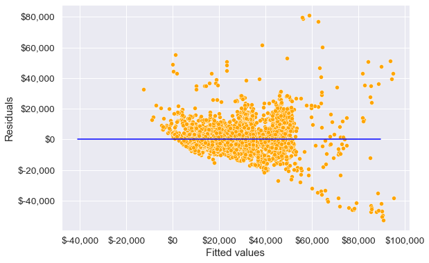

We see that the variance of errors seems to increase with increase in the fitted values. In such a case a log transformation of the response can resolve the issue to some extent. This is because a log transformation will result in a higher shrinkage of larger values.

#Model with an interaction term and a variable transformation term
ols_object = smf.ols(formula = 'np.log(price)~(year+engineSize+mileage+mpg)**2+I(mileage**2)', data = train)
model_log = ols_object.fit()
model_log.summary()

OLS Regression Results
Dep. Variable:	np.log(price)	R-squared:	0.803
Model:	OLS	Adj. R-squared:	0.803
Method:	Least Squares	F-statistic:	1834.
Date:	Wed, 25 Jan 2023	Prob (F-statistic):	0.00
Time:	11:37:55	Log-Likelihood:	-1173.8
No. Observations:	4960	AIC:	2372.
Df Residuals:	4948	BIC:	2450.
Df Model:	11
Covariance Type:	nonrobust

	coef	std err	t	P>\|t\|	[0.025	0.975]
Intercept	-238.2125	25.790	-9.237	0.000	-288.773	-187.652
year	0.1227	0.013	9.608	0.000	0.098	0.148
engineSize	13.8349	5.795	2.387	0.017	2.475	25.195
mileage	0.0005	0.000	3.837	0.000	0.000	0.001
mpg	-1.2446	0.345	-3.610	0.000	-1.921	-0.569
year:engineSize	-0.0067	0.003	-2.324	0.020	-0.012	-0.001
year:mileage	-2.67e-07	6.8e-08	-3.923	0.000	-4e-07	-1.34e-07
year:mpg	0.0006	0.000	3.591	0.000	0.000	0.001
engineSize:mileage	-2.668e-07	4.08e-07	-0.654	0.513	-1.07e-06	5.33e-07
engineSize:mpg	0.0028	0.000	6.842	0.000	0.002	0.004
mileage:mpg	7.235e-08	1.79e-08	4.036	0.000	3.72e-08	1.08e-07
I(mileage ** 2)	1.828e-11	5.64e-12	3.240	0.001	7.22e-12	2.93e-11

Omnibus:	711.515	Durbin-Watson:	0.498
Prob(Omnibus):	0.000	Jarque-Bera (JB):	2545.807
Skew:	0.699	Prob(JB):	0.00
Kurtosis:	6.220	Cond. No.	1.73e+13

Note that the coefficient of year turns out to be significant (at 5% significance level), unlike in the previous model. Intuitively, the coefficient of year should have been significant, as year has the highest linear correlation of 50% with car price.

Although the R-squared has increased as compared to the previous model, violation of this assumption does not cause bias in the regression coefficients. Thus, there may not be a large improvement in the model fit, unless we add predictor(s) to address heteroscedasticity.

Let us check the constant variance assumption again.

#Plotting residuals vs fitted values
sns.scatterplot(x = (model_log.fittedvalues), y=(model_log.resid),color = 'orange')
sns.lineplot(x = [model_log.fittedvalues.min(),model_log.fittedvalues.max()],y = [0,0],color = 'blue')
plt.xlabel('Fitted values')
plt.ylabel('Residuals')

Text(0, 0.5, 'Residuals')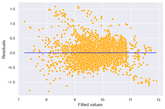

Now we observe that the constant variance assumption is satisfied. Let us see the RMSE of this model on test data.

#Computing RMSE on test data
pred_price_log = model_log.predict(testf)
np.sqrt(((testp.price - np.exp(pred_price_log))**2).mean())

9094.209503063496

Note that the RMSE of the log-transformed model has increased as compared to the model without transformation. Does it mean the log-transformed model is less accurate?

#Computing MAE on test data
pred_price_log = model_log.predict(testf)
((np.abs(testp.price - np.exp(pred_price_log))).mean())

5268.398904745121

Although the RMSE has increased a bit for the log-transformed model, the MAE has reduced. This means the log-transformed model does a bit worse on reducing relatively large errors, but does better in reducing the absolute errors on an average.

#Comparing errors of the log-transformed model with the previous model
err = np.abs(testp.price - pred_price)
err_log = np.abs(testp.price - np.exp(pred_price_log))
sns.scatterplot(x = err,y = err_log, color = 'orange')
sns.lineplot(x = [0,100000], y = [0,100000], color = 'blue')
np.sum(err_log<err)/len(err)

0.5572604790419161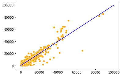

For 56% of the cars, the log transformed makes a more accurate prediction than the previous model, which is another criterion based on which the log-transformed model is more accurate. However, the conclusion based on RMSE is different. This is because RMSE can be influenced by a few large errors. Thus, RMSE, though sometimes appropriate than other criteria, should not be used as the sole measure to compare the accuracy of models.

#Visualizing the distribution of price and log(price)
fig = plt.figure()
fig.subplots_adjust(hspace=0.4, wspace=0.2)
sns.set(rc = {'figure.figsize':(20,12)})
sns.set(font_scale = 2)
ax = fig.add_subplot(2, 2, 1)
sns.histplot(train.price,kde=True)
ax.set(xlabel='price', ylabel='Count')
ax = fig.add_subplot(2, 2, 2)
sns.histplot(np.log(train.price),kde=True)
ax.set(xlabel='log price', ylabel='Count')

[Text(0.5, 0, 'log price'), Text(0, 0.5, 'Count')]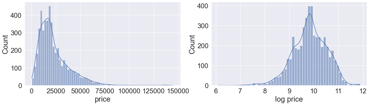

We can see that the log transformation shrinked the higher values of price, making its distribution closer to normal.

Note that heteroscedasticity can also occur due to model misspecification, i.e., in case of missing predictor(s). Some of the cars are too expensive, which makes the price distribution skewed. Perhaps, the price of expensive cars could be better explained by the car model, a predictor that is missing in the current model.