2 Multiple Linear Regression

Read section 3.2 of the book before using these notes.

Note that in this course, lecture notes are not sufficient, you must read the book for better understanding. Lecture notes are just implementing the concepts of the book on a dataset, but not explaining the concepts elaborately.

2.1 Multiple Linear Regression

import pandas as pd
import numpy as np
import statsmodels.formula.api as smf
import seaborn as sns
import matplotlib.pyplot as plt

Develop a multiple linear regression model that predicts car price based on engine size, year, mileage, and mpg. Datasets to be used: Car_features_train.csv, Car_prices_train.csv

trainf = pd.read_csv('./Datasets/Car_features_train.csv')
trainp = pd.read_csv('./Datasets/Car_prices_train.csv')
train = pd.merge(trainf,trainp)
train.head()

	carID	brand	model	year	transmission	mileage	fuelType	tax	mpg	engineSize	price
0	18473	bmw	6 Series	2020	Semi-Auto	11	Diesel	145	53.3282	3.0	37980
1	15064	bmw	6 Series	2019	Semi-Auto	10813	Diesel	145	53.0430	3.0	33980
2	18268	bmw	6 Series	2020	Semi-Auto	6	Diesel	145	53.4379	3.0	36850
3	18480	bmw	6 Series	2017	Semi-Auto	18895	Diesel	145	51.5140	3.0	25998
4	18492	bmw	6 Series	2015	Automatic	62953	Diesel	160	51.4903	3.0	18990

#Using the ols function to create an ols object. 'ols' stands for 'Ordinary least squares'
ols_object = smf.ols(formula = 'price~year+mileage+mpg+engineSize', data = train)
model = ols_object.fit()
model.summary()

OLS Regression Results
Dep. Variable:	price	R-squared:	0.660
Model:	OLS	Adj. R-squared:	0.660
Method:	Least Squares	F-statistic:	2410.
Date:	Tue, 27 Dec 2022	Prob (F-statistic):	0.00
Time:	01:07:25	Log-Likelihood:	-52497.
No. Observations:	4960	AIC:	1.050e+05
Df Residuals:	4955	BIC:	1.050e+05
Df Model:	4
Covariance Type:	nonrobust

	coef	std err	t	P>\|t\|	[0.025	0.975]
Intercept	-3.661e+06	1.49e+05	-24.593	0.000	-3.95e+06	-3.37e+06
year	1817.7366	73.751	24.647	0.000	1673.151	1962.322
mileage	-0.1474	0.009	-16.817	0.000	-0.165	-0.130
mpg	-79.3126	9.338	-8.493	0.000	-97.620	-61.006
engineSize	1.218e+04	189.969	64.107	0.000	1.18e+04	1.26e+04

Omnibus:	2450.973	Durbin-Watson:	0.541
Prob(Omnibus):	0.000	Jarque-Bera (JB):	31060.548
Skew:	2.045	Prob(JB):	0.00
Kurtosis:	14.557	Cond. No.	3.83e+07

Notes:
[1] Standard Errors assume that the covariance matrix of the errors is correctly specified.
[2] The condition number is large, 3.83e+07. This might indicate that there are
strong multicollinearity or other numerical problems.

The model equation is: estimated car price = -3.661e6 + 1818 * year -0.15 * mileage - 79.31 * mpg + 12180 * engineSize

Predict the car price for the cars in the test dataset. Datasets to be used: Car_features_test.csv, Car_prices_test.csv

testf = pd.read_csv('./Datasets/Car_features_test.csv')
testp = pd.read_csv('./Datasets/Car_prices_test.csv')

#Using the predict() function associated with the 'model' object to make predictions of car price on test (unknown) data
pred_price = model.predict(testf)#Note that the predict() function finds the predictor 'engineSize' in the testf dataframe, and plugs its values in the regression equation for prediction.

Make a visualization that compares the predicted car prices with the actual car prices

sns.scatterplot(x = testp.price, y = pred_price)
#In case of a perfect prediction, all the points must lie on the line x = y.
sns.lineplot(x = [0,testp.price.max()], y = [0,testp.price.max()],color='orange') #Plotting the line x = y.
plt.xlabel('Actual price')
plt.ylabel('Predicted price')

Text(0, 0.5, 'Predicted price')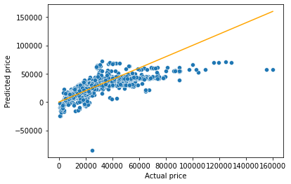

The prediction looks better as compared to the one with simple linear regression. This is because we have four predictors to help explain the variation in car price, instead of just one in the case of simple linear regression. Also, all the predictors have a significant relationship with price as evident from their p-values. Thus, all four of them are contributing in explaining the variation. Note the higher values of R2 as compared to the one in the case of simple linear regression.

What is the RMSE of the predicted car price?

np.sqrt(((testp.price - pred_price)**2).mean())

9956.82497993548

What is the residual standard error based on the training data?

np.sqrt(model.mse_resid)

9563.74782917604

sns.scatterplot(x = model.fittedvalues, y=model.resid,color = 'orange')
sns.lineplot(x = [pred_price.min(),pred_price.max()],y = [0,0],color = 'blue')
plt.xlabel('Predicted price')
plt.ylabel('Residual')

Text(0, 0.5, 'Residual')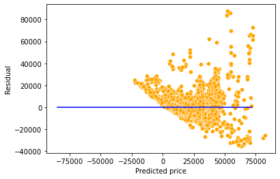

Will the explained variation (R-squared) in car price always increase if we add a variable?

Should we keep on adding variables as long as the explained variation (R-squared) is increasing?

#Using the ols function to create an ols object. 'ols' stands for 'Ordinary least squares'
np.random.seed(1)
train['rand_col'] = np.random.rand(train.shape[0])
ols_object = smf.ols(formula = 'price~year+mileage+mpg+engineSize+rand_col', data = train)
model = ols_object.fit()
model.summary()

OLS Regression Results
Dep. Variable:	price	R-squared:	0.661
Model:	OLS	Adj. R-squared:	0.660
Method:	Least Squares	F-statistic:	1928.
Date:	Tue, 27 Dec 2022	Prob (F-statistic):	0.00
Time:	01:07:38	Log-Likelihood:	-52497.
No. Observations:	4960	AIC:	1.050e+05
Df Residuals:	4954	BIC:	1.050e+05
Df Model:	5
Covariance Type:	nonrobust

	coef	std err	t	P>\|t\|	[0.025	0.975]
Intercept	-3.662e+06	1.49e+05	-24.600	0.000	-3.95e+06	-3.37e+06
year	1818.1672	73.753	24.652	0.000	1673.578	1962.756
mileage	-0.1474	0.009	-16.809	0.000	-0.165	-0.130
mpg	-79.2837	9.338	-8.490	0.000	-97.591	-60.976
engineSize	1.218e+04	189.972	64.109	0.000	1.18e+04	1.26e+04
rand_col	451.1226	471.897	0.956	0.339	-474.004	1376.249

Omnibus:	2451.728	Durbin-Watson:	0.541
Prob(Omnibus):	0.000	Jarque-Bera (JB):	31040.331
Skew:	2.046	Prob(JB):	0.00
Kurtosis:	14.552	Cond. No.	3.83e+07

Adding a variable with random values to the model (rand_col) increased the explained variation (R-squared). This is because the model has one more parameter to tune to reduce the residual squared error (RSS). However, the p-value of rand_col suggests that its coefficient is zero. Thus, using the model with rand_col may give poorer performance on unknown data, as compared to the model without rand_col. This implies that it is not a good idea to blindly add variables in the model to increase R-squared.