#loading libraries
library(ggplot2)7 Variable interactions & Qualitative predictors
In this chapter, we’ll introduce interactions, and then develop and interpret models with interactions among quantitative predictors, and interactions between quantitative and qualitative predictors.
7.1 Interaction model
Let us consider the file car_data.csv.
# Reading data
car_data <- read.csv('./Datasets/car_data.csv')
head(car_data)
carID brand model year transmission mileage fuelType tax mpg
1 12002 hyundi Santa Fe 2017 Semi-Auto 32467 Diesel 235 42.9709
2 12003 vw Arteon 2019 Automatic 1555 Petrol 145 40.5071
3 12005 toyota Verso 2003 Automatic 104000 Petrol 300 34.5227
4 12006 ford Grand C-MAX 2018 Manual 5113 Petrol 145 47.6225
5 12007 bmw X6 2019 Automatic 9010 Diesel 145 35.2224
6 12008 toyota Prius 2016 Automatic 32853 Hybrid 10 63.8371
engineSize price
1 2.2 18991
2 1.5 22500
3 1.8 2395
4 1.0 14000
5 3.0 58700
6 1.8 22995In an additive model, we assume that the association between a predictor \(X_j\) and response \(Y\) does not depend on the value of other predictors. For example, consider the multiple linear regression model below.
# Additive model
additive_model <- lm(price~year+engineSize+mileage+mpg, data = car_data)
summary(additive_model)
Call:
lm(formula = price ~ year + engineSize + mileage + mpg, data = car_data)

Residuals:
   Min     1Q Median     3Q    Max
-35346  -5131  -1605   2854  87509

Coefficients:
              Estimate Std. Error t value Pr(>|t|)
(Intercept) -3.661e+06  1.489e+05 -24.593   <2e-16 ***
year         1.818e+03  7.375e+01  24.647   <2e-16 ***
engineSize   1.218e+04  1.900e+02  64.107   <2e-16 ***
mileage     -1.474e-01  8.768e-03 -16.817   <2e-16 ***
mpg         -7.931e+01  9.338e+00  -8.493   <2e-16 ***
---
Signif. codes:  0 '***' 0.001 '**' 0.01 '*' 0.05 '.' 0.1 ' ' 1

Residual standard error: 9564 on 4955 degrees of freedom
Multiple R-squared:  0.6605,    Adjusted R-squared:  0.6602
F-statistic:  2410 on 4 and 4955 DF,  p-value: < 2.2e-16
The above model assumes that the average increase in price associated with a unit increase in engineSize is always $12,180, regardless of the value of other predictors. However, this assumption may be incorrect.
7.2 Interaction between continuous predictors
We can relax this assumption by considering another predictor, called an interaction term. Let us assume that the average increase in price associated with a one-unit increase in engineSize depends on the model year of the car. In other words, there is an interaction between engineSize and year. This interaction can be included as a predictor, which is the product of engineSize and year. Note that there are several possible interactions that we can consider. Here the interaction between engineSize and year is just an example.
# Interaction model
interaction_model <- lm(price~year*engineSize+mileage+mpg, data = car_data)
summary(interaction_model)
Call:
lm(formula = price ~ year * engineSize + mileage + mpg, data = car_data)

Residuals:
   Min     1Q Median     3Q    Max
-40479  -4929  -1548   2864  85271

Coefficients:
                  Estimate Std. Error t value Pr(>|t|)
(Intercept)      5.606e+05  2.737e+05   2.048   0.0406 *
year            -2.754e+02  1.357e+02  -2.029   0.0425 *
engineSize      -1.796e+06  9.968e+04 -18.019   <2e-16 ***
mileage         -1.525e-01  8.496e-03 -17.954   <2e-16 ***
mpg             -8.434e+01  9.048e+00  -9.322   <2e-16 ***
year:engineSize  8.968e+02  4.943e+01  18.142   <2e-16 ***
---
Signif. codes:  0 '***' 0.001 '**' 0.01 '*' 0.05 '.' 0.1 ' ' 1

Residual standard error: 9262 on 4954 degrees of freedom
Multiple R-squared:  0.6816,    Adjusted R-squared:  0.6813
F-statistic:  2121 on 5 and 4954 DF,  p-value: < 2.2e-16
Note that the \(R^2\) has increased as compared to the additive model, since we added a predictor.
The model equation is:
price = \(\beta_0\) + \(\beta_1\)year + \(\beta_2\)engineSize + \(\beta_3\)(year \(\times\) engineSize) + \(\beta_4\)mileage + \(\beta_5\)mpg, or
price = \(\beta_0\) + \(\beta_1\)year + (\(\beta_2+\beta_3\)year) \(\times\) engineSize + \(\beta_4\)mileage + \(\beta_5\)mpg, or
price = \(\beta_0 + \beta_1\)year + \(\tilde \beta\)engineSize + \(\beta_4\)mileage + \(\beta_5\)mpg,
Since \(\tilde \beta\) is a function of year, the association between engineSize and price is no longer a constant. A change in the value of year will change the association between price and engineSize.
Substituting the values of the coefficients:
price = 5.606e5 - 275.3833year + (-1.796e6+896.7687year)engineSize -0.1525mileage -84.3417mpg
Thus, for cars launched in the year 2010, the average increase in price for one liter increase in engine size is -1.796e6 + 896.7687 * 2010 \(\approx\) $6,500, assuming all the other predictors are constant. However, for cars launched in the year 2020, the average increase in price for one liter increase in engine size is -1.796e6 + 896.7687*2020 \(\approx\) $15,500 , assuming all the other predictors are constant.
Similarly, the equation can be re-arranged as:
price = 5.606e5 +(-275.3833+896.7687engineSize)year -1.796e6engineSize -0.1525mileage -84.3417mpg
Thus, for cars with an engine size of 2 litres, the average increase in price for a one year newer model is -275.3833+896.7687 * 2 \(\approx\) $1500, assuming all the other predictors are constant. However, for cars with an engine size of 3 litres, the average increase in price for a one year newer model is -275.3833+896.7687 * 3 \(\approx\) $2400, assuming all the other predictors are constant.
7.3 Qualitative predictors
Let us develop a model for predicting price based on engineSize and the qualitative predictor transmission.
#checking the distribution of values of transmission
table(car_data$transmission)
Automatic    Manual     Other Semi-Auto
     1660      1948         1      1351
Note that the Other category of the variable transmission contains only a single observation, which is likely to be insufficient to train the model. We’ll remove that observation from the car data. Another option may be to combine the observation in the Other category with the nearest category, and keep it in the data.
car_data = car_data[car_data$transmission!='Other',]qual_pred_model <- lm(price~engineSize+transmission, data = car_data)
summary(qual_pred_model)
Call:
lm(formula = price ~ engineSize + transmission, data = car_data)

Residuals:
   Min     1Q Median     3Q    Max
-47181  -6726  -1145   5204  95998

Coefficients:
                      Estimate Std. Error t value Pr(>|t|)
(Intercept)             3042.7      661.2   4.602 4.29e-06 ***
engineSize             10226.8      247.5  41.323  < 2e-16 ***
transmissionManual     -6770.6      442.1 -15.314  < 2e-16 ***
transmissionSemi-Auto   4994.3      443.0  11.274  < 2e-16 ***
---
Signif. codes:  0 '***' 0.001 '**' 0.01 '*' 0.05 '.' 0.1 ' ' 1

Residual standard error: 12080 on 4955 degrees of freedom
Multiple R-squared:  0.4587,    Adjusted R-squared:  0.4584
F-statistic:  1400 on 3 and 4955 DF,  p-value: < 2.2e-16
Note that there is no coefficient for the Automatic level of the variable Transmission. If a car doesn’t have Manual or Semi-Automatic transmission, then it has an Automatic transmission. Thus, the coefficient of Automatic will be redundant, and the dummy variable corresponding to Automatic transmission is dropped from the model.
The level of the categorical variable that is dropped from the model is called the baseline level. Here Automatic transmission is the baseline level. The coefficients of other levels of transmission should be interpreted with respect to the baseline level.
Q: Interpret the intercept term.
Ans: For the hypothetical scenario of a car with zero engine size and Automatic transmission, the estimated mean car price is \(\approx\) $3042.
Q: Interpret the coefficient of transmissionManual.
Ans: The estimated mean price of a car with manual transmission is \(\approx\) $6770 less than that of a car with Automatic transmission.
Let us visualize the developed model.
colors <- c("Automatic" = "red", "Manual" = "blue", "Semi-Automatic" = "green")

coefs <- qual_pred_model$coefficients
x <- car_data$engineSize
ggplot(data = car_data, aes(x = engineSize))+
  geom_line(aes(y = coefs['(Intercept)']+x*coefs['engineSize'], color = 'Automatic'))+
  geom_line(aes(y = coefs['(Intercept)']+x*coefs['engineSize']+coefs['transmissionManual'], color = 'Manual'))+
  geom_line(aes(y = coefs['(Intercept)']+x*coefs['engineSize']+coefs['transmissionSemi-Auto'], color = 'Semi-Automatic'))+
  theme(legend.title = element_blank(),
        legend.position = c(0.15,0.85))+
  labs(
    y = 'Predicted car price',
    x = 'Engine size (in litre)'
  )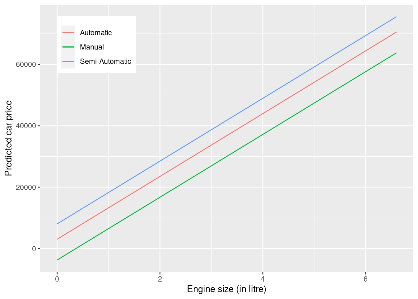
Based on the developed model, for a given engine size, the car with a semi-automatic transmission is estimated to be the most expensive on average, while the car with a manual transmission is estimated to be the least expensive on average.
Q: What is the expected difference between the price of a car with Manual Transmission and a car with a Semi-Automatic transmission?
A: The expected difference is \(\hat{\beta}_{I(Tranmission = Manual)} - \hat{\beta}_{I(Tranmission = Semi-Automatic)} = -6770.6 - 4994.3 = -\$11,764.9\)
Q: Find the 95% confidence interal for the point estimate obtained in the previous question.
A: Let us compute the standard error of the point estimate:
\(Var(\hat{\beta}_{I(Tranmission = Manual)} - \hat{\beta}_{I(Tranmission = Semi-Automatic)}) = Var(\hat{\beta}_{I(Tranmission = Manual)}) + Var(\hat{\beta}_{I(Tranmission = Semi-Automatic)}) - 2CoVar(\hat{\beta}_{I(Tranmission = Manual)}, \hat{\beta}_{I(Tranmission = Semi-Automatic)})\)
The R function vcov() provides the variance-covariance matrix of the regression coefficients, which can be used the evaluate the above expression.
# Variance-covariance matrix of the regression coefficients
vcov_matrix <- vcov(qual_pred_model)
We’ll use the variance-covariance matrix to compute the variance of the point estimate, and use the variance to compute the confidence interval:
# Variance of the point estimate
variance_point_estimate = vcov_matrix[3,3] + vcov_matrix[4,4] - 2*vcov_matrix[3,4]

# Standard deviation of the point estimate
std_point_estimate = sqrt(variance_point_estimate)

# Upper bound of the 95% CI of the point estimate
UB <- -11764.9 + std_point_estimate*qt(0.975, 4959-4)
print(paste0("Upper bound = ",UB))
[1] "Upper bound = -10837.3953392871"LB <- -11764.9 - std_point_estimate*qt(0.975, 4959-4)
print(paste0("Lower bound = ", LB))[1] "Lower bound = -12692.4046607129"The 95% confidence interval is: [-$10.8k,-$12.7k].
7.4 Interaction between qualitative and continuous predictors
Note that the qualitative predictor leads to fitting 3 parallel lines to the data, as there are 3 categories.
However, note that we have made the constant association assumption. The fact that the lines are parallel means that the average increase in car price for one litre increase in engine size does not depend on the type of transmission. This represents a potentially serious limitation of the model, since in fact a change in engine size may have a very different association on the price of an automatic car versus a semi-automatic or manual car.
This limitation can be addressed by adding an interaction variable, which is the product of engineSize and the dummy variables for semi-automatic and manual transmissions.
qual_pred_int_model <- lm(price~engineSize*transmission, data = car_data)
summary(qual_pred_int_model)
Call:
lm(formula = price ~ engineSize * transmission, data = car_data)

Residuals:
   Min     1Q Median     3Q    Max
-56431  -6453  -1033   5184  96479

Coefficients:
                                 Estimate Std. Error t value Pr(>|t|)
(Intercept)                        3754.7      895.2   4.194 2.79e-05 ***
engineSize                         9928.6      354.5  28.006  < 2e-16 ***
transmissionManual                 1768.6     1294.1   1.367 0.171786
transmissionSemi-Auto             -5282.7     1416.5  -3.729 0.000194 ***
engineSize:transmissionManual     -5285.9      646.2  -8.180 3.57e-16 ***
engineSize:transmissionSemi-Auto   4162.2      552.6   7.532 5.90e-14 ***
---
Signif. codes:  0 '***' 0.001 '**' 0.01 '*' 0.05 '.' 0.1 ' ' 1

Residual standard error: 11850 on 4953 degrees of freedom
Multiple R-squared:  0.4788,    Adjusted R-squared:  0.4782
F-statistic: 909.9 on 5 and 4953 DF,  p-value: < 2.2e-16
The model equation for the model with interactions is:
Automatic transmission: price = 3754.7238 + 9928.6082engineSize,
Semi-Automatic transmission: price = 3754.7238 + 9928.6082engineSize + (-5282.7164+4162.2428engineSize),
Manual transmission: price = 3754.7238 + 9928.6082engineSize +(1768.5856-5285.9059engineSize), or
Automatic transmission: price = 3754.7238 + 9928.6082engineSize,
Semi-Automatic transmission: price = -1527 + 7046engineSize,
Manual transmission: price = 5523 + 4642engineSize.
Q: Interpret the coefficient of manual tranmission, i.e., the coefficient of transmissionManual.
A: For the hypothetical scenario of a car with zero engine size,the estimated mean price of a car with Manual transmission is \(\approx\) $1768 more than the estimated mean price of a car with Automatic transmission.
Q: Interpret the coefficient of the interaction between engine size and manual transmission, i.e., the coefficient of engineSize:transmissionManual.
A: For a unit (or a litre) increase in engineSize , the increase in estimated mean price of a car with Manual transmission is \(\approx\) $5285 less than the increase in estimated mean price of a car with Automatic transmission.
colors <- c("Automatic" = "red", "Manual" = "blue", "Semi-Automatic" = "green")

coefs <- qual_pred_int_model$coefficients
x <- car_data$engineSize
ggplot(data = car_data, aes(x = engineSize))+
  geom_line(aes(y = coefs['(Intercept)']+x*coefs['engineSize'], color = 'Automatic'))+
  geom_line(aes(y = coefs['(Intercept)']+x*coefs['engineSize']+coefs['transmissionManual']+x*coefs['engineSize:transmissionManual'], color = 'Manual'))+
  geom_line(aes(y = coefs['(Intercept)']+x*coefs['engineSize']+coefs['transmissionSemi-Auto']+x*coefs['engineSize:transmissionSemi-Auto'], color = 'Semi-Automatic'))+
  theme(legend.title = element_blank(),
        legend.position = c(0.15,0.85))+
  labs(
    y = 'Predicted car price',
    x = 'Engine size (in litre)'
  )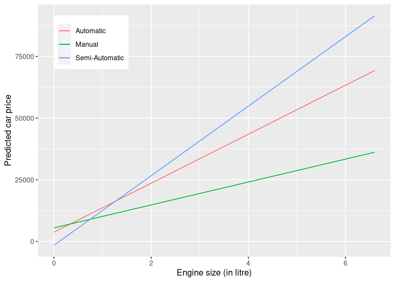
Note the interaction term adds flexibility to the model.
The slope of the regression line for semi-automatic cars is the largest. This suggests that increase in engine size is associated with a higher increase in car price for semi-automatic cars, as compared to other cars.