library(ISLR) #for the dataset
library(ggplot2) #for making plots
library(lmtest) #for bptest()
library(MASS) #for boxcox()4 Diagnostics and Remedial measures (SLR)
Let us consider the Auto dataset from the ISLR library. The library is related to the book Introduction to Statistical Learning
4.1 Loading libraries
4.2 Reading data
auto_data <- Auto4.3 Developing model
Suppose we wish to predict mpg based on horsepower.
linear_model <- lm(mpg~horsepower, data = auto_data)4.4 Model fit
Let us visualize the model fit to the data.
ggplot(data = auto_data, aes(x = horsepower, y = mpg))+
  geom_point()+
  geom_smooth(method = "lm")
`geom_smooth()` using formula = 'y ~ x'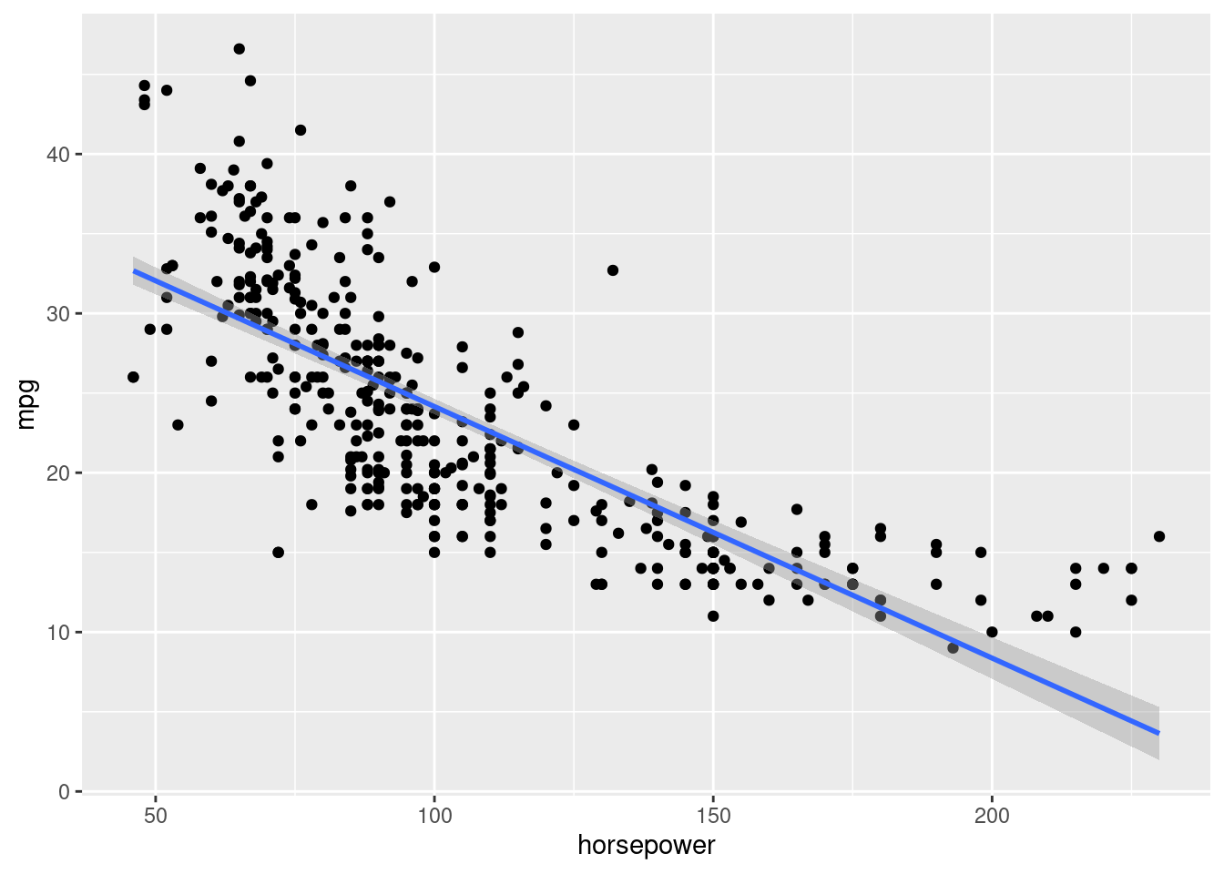
The plot indicates that a quadratic relationship between mpg and horsepower may be more appropriate.
4.5 Diagnostic plots & statistical tests
Let us make diagnostic plots that help us check the model assumptions.
par(mfrow = c(2,2))
plot(linear_model)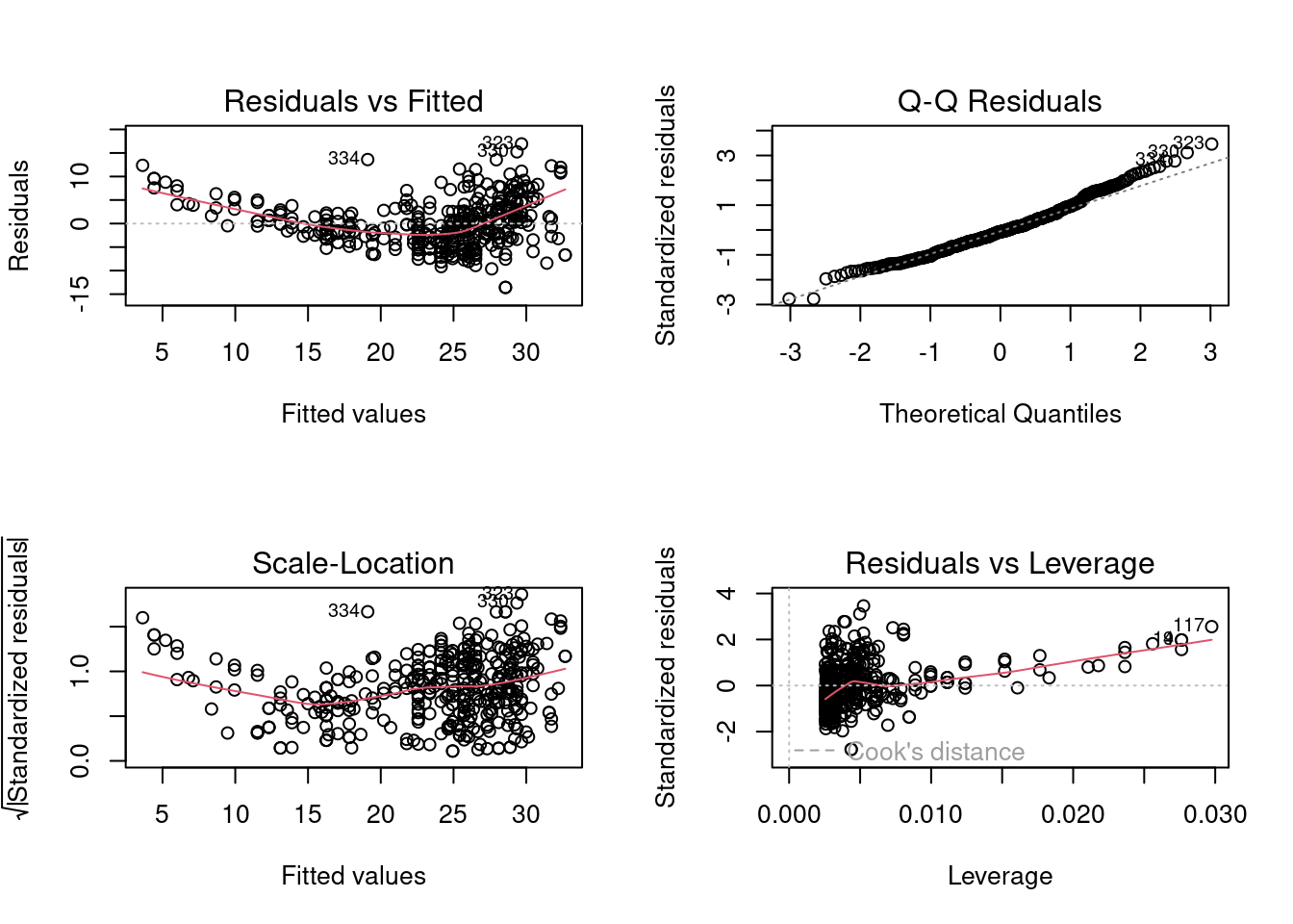
4.5.1 Linear relationship
4.5.1.1 Visual check
We can check the linearity assumption visually by analyzing the plot of residuals against fitted values. The plot indicates that a quadratic relationship between the response and the predictor may be more appropriate than a linear one.
4.5.1.2 Statistical test
We’ll use the F test for lack of fit to check the linearity assumption
#Full model
full_model <- lm(mpg~as.factor(horsepower), data = auto_data)
# F test for lack of fit
anova(linear_model, full_model)Analysis of Variance Table
Model 1: mpg ~ horsepower
Model 2: mpg ~ as.factor(horsepower)
Res.Df RSS Df Sum of Sq F Pr(>F)
1 390 9385.9
2 299 4702.8 91 4683.1 3.272 1.125e-14 ***
---
Signif. codes: 0 '***' 0.001 '**' 0.01 '*' 0.05 '.' 0.1 ' ' 1As expected based on the visual check, the linear model fails the linearity test with a very low \(p\)-value of the order of \(10^{-14}\). Thus, we conclude that relationship is non-linear.
4.5.2 Constant variance (Homoscedasticity)
4.5.2.1 Visual check
The plot of the residuals against fitted values indicates that the error variance is increasing with increasing values of predicted mpg or decreasing horsepower. Thus, there seems to be heteroscedasticity.
4.5.2.2 Statistical test
Breusch-Pagan test
Let us conduct the Breusch-Pagan test for homoscedasticity. This is a large sample test, which assumes that the error terms are independent and normally distruted, and that the variance of of the error term \(\epsilon_i\), denoted by \(\sigma_i^2\), is related to the level of the predictor \(X\) in the following way:
\(\log(\sigma_i^2) = \gamma_0 + \gamma_1X_i\).
This implies that \(\sigma_i^2\) either increases or decreases with the level of \(X\). Constant error variance corresponds to \(\gamma_1 = 0\). The hypotheses for the test are:
\(H_0: \gamma_1 = 0\) \(H_a: \gamma_1 \ne 0\)
bptest(linear_model)
    studentized Breusch-Pagan test

data:  linear_model
BP = 8.7535, df = 1, p-value = 0.00309
As expected based on the visual check, the model fails the homoscedasticity with a low \(p\)-value of 0.3%.
Brown-Forsythe test
To conduct the Brown-Forsythe test, we divide the data into two groups, based on the predictor \(X\). If the error variance is not constant, the residuals in one group will tend to be more variable than those in the other group. The test consists of a two-sample \(t\)-test to determine whether the mean of the absolute deviations from the median residual of one group differs significantly from the mean of the absolute deviations from the median residual of the other group.
#Break the residuals into 2 groups
residuals_group1 <- linear_model$residuals[auto_data$horsepower<=100]
residuals_group2 <- linear_model$residuals[auto_data$horsepower>100]
#Obtain the median of each group
median_group1 <- median(residuals_group1)
median_group2 <- median(residuals_group2)#Two-sample t-test
t.test(abs(residuals_group1-median_group1), abs(residuals_group2-median_group2), var.equal = TRUE)
    Two Sample t-test

data:  abs(residuals_group1 - median_group1) and abs(residuals_group2 - median_group2)
t = 4.4039, df = 390, p-value = 1.375e-05
alternative hypothesis: true difference in means is not equal to 0
95 percent confidence interval:
 0.7738625 2.0220633
sample estimates:
mean of x mean of y
 4.308698  2.910735
Brown-Forsythe test also shows that there is heteroscedasticity.
4.5.3 Normality of error terms
4.5.3.1 Visual check
The QQ plot indicates that the distribution of the residuals is slightly right-skewed. This right-skew can be visualized by making a histogram or a density plot of residuals:
par(mfrow = c(1,1))
hist(linear_model$residuals, breaks = 20, prob = TRUE)
lines(density(linear_model$residuals), col = 'blue')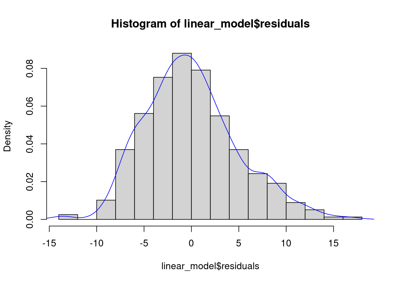
4.5.3.2 Statistical test
shapiro.test(linear_model$residuals)
    Shapiro-Wilk normality test

data:  linear_model$residuals
W = 0.98207, p-value = 8.734e-05
As expected based on the visual check, the model fails the test for normal distribution of error terms with a low \(p\)-value of the order of \(10^{-5}\).
4.5.4 Independence of error terms
This test is relevant if there is an order in the data, i.e., if the observations can be arranged based on time, space, etc. In the current example, there is no order, and so this test is not relevant.
4.6 Remedial Measures
If the linear relationship assumption violated, it results in biased estimates of the regression coefficients resulting in a biased prediction. As the estimates are biased, their variance estimates may also be inaccurate. Thus, this is a very important assumption as it leads to inaccuracies in both point estimates and statistical inference.
If the homoscedasticity assumption is violated, but the linear relationship assumption holds, the OLS estimates are still unbiased resulting in an unbiased prediction. However, their standard error estimates are likely to be inaccurate.
If the assumption regarding the normal distribution of errors is violated, the OLS estimates are still BLUE (Best linear unbiased estimates). The confidence interval for a point estimate, though effected, is robust to departures from normality for large sample sizes. However, the prediction interval is sensitive to the same.
Our model above (linear_model) violates all the three assumptions.
Note that there is no one unique way of fixing all the model assumption violations. Its an iterative process, and there is some trial and error involved. Two different approaches may lead to two different models, and both models may be more or less similar (in terms of point estimates / inference)
4.6.1 Addressing linear relationship assumption violation
Let us address the linear relationship assumption first.
As indicated in the diagnostic plots, the relationship between \(X\) and \(Y\) seemed to be quadratic. We’ll change the simple linear regression model to the following linear regression model, where \(Y\) and \(X\) have a quadratic relationship:
\(Y_i = \beta_0 + \beta_1X_i + \beta_2X_i^2\)
Let us fit the above model to the data:
quadratic_model <- lm(mpg~horsepower + I(horsepower**2), data = auto_data)Note that in the formula specified within the lm() function, the I() operator isolates or insulates the contents within I(…) from the regular formula operators. Without the I() operator, horsepower**2 will be treated as the interaction of horsepower with itself, which is horsepower. Thus, to add the square of horsepower as a separate predictor, we need to use the I() operator.
After every transformation or remedial measure, we should diagnoze the model to check the model assumptions are satisfied.
par(mfrow=c(2,2))
plot(quadratic_model)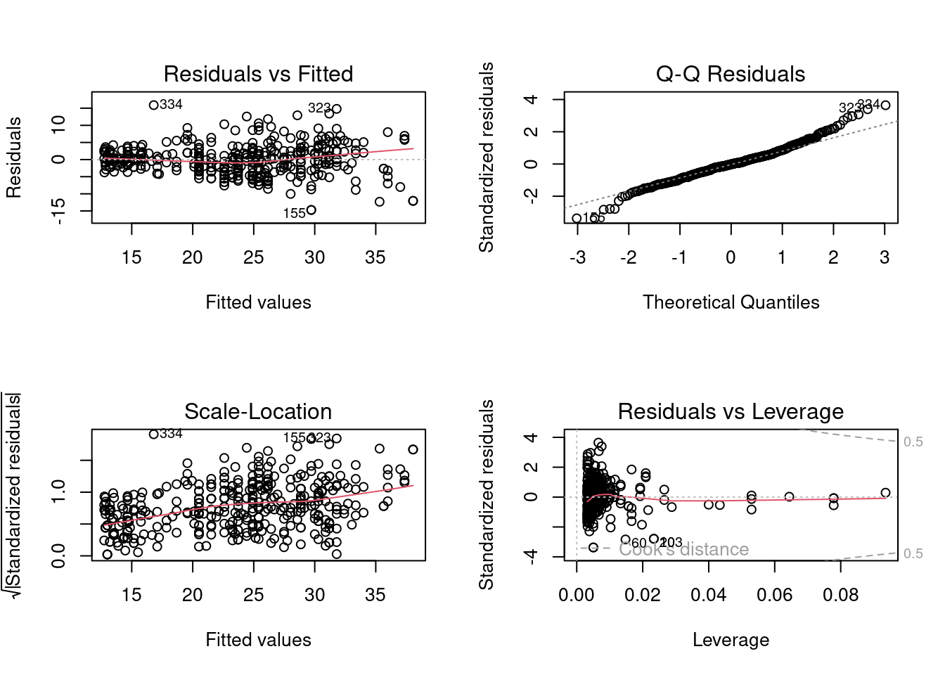
We observe that the departure from the linear relationship assumption has been reduced. However, there still seems to be heteroscedasticity and non-normal error terms. Let us verify this with statistical tests.
#F test for lack of fit
anova(quadratic_model, full_model)
Analysis of Variance Table
Model 1: mpg ~ horsepower + I(horsepower^2)
Model 2: mpg ~ as.factor(horsepower)
Res.Df RSS Df Sum of Sq F Pr(>F)
1 389 7442.0
2 299 4702.8 90 2739.3 1.9351 1.897e-05 ***
---
Signif. codes: 0 '***' 0.001 '**' 0.01 '*' 0.05 '.' 0.1 ' ' 1Even though the model still fails the linearity test, the extent of violation is reduced as the \(p\)-value is now of the order of \(10^{-5}\) instead of \(10^{-14}\).
# Breusch-Pagan test
bptest(quadratic_model)
    studentized Breusch-Pagan test

data:  quadratic_model
BP = 34.528, df = 2, p-value = 3.179e-08
The quadratic model has a more severe heteroscedasticity as compared to the linear model based on the \(p\)-value.
shapiro.test(quadratic_model$residuals)
    Shapiro-Wilk normality test

data:  quadratic_model$residuals
W = 0.98268, p-value = 0.0001214
The severity of departure from normality has been reduced in the quadratic model.
4.6.2 Addressing heteroscedasticity
Let us address the heteroscedasticity assumption.
We can see from the diagnostic plot of the quadratic model that the error variance is higher for higher fitted values. A possible way to resolve this is to transform the response \(Y\) using a concave function such as log(\(Y\)) or \(\sqrt{Y}\). Such a transformation results in a greater amount of shrinkage of the larger responses, leading to a reduction in heteroscedasticity. Let us try the log(\(Y\)) transformation to address heteroscedasticity.
log_model <- lm(log(mpg)~horsepower+I(horsepower**2), data = auto_data)
par(mfrow=c(2,2))
plot(log_model)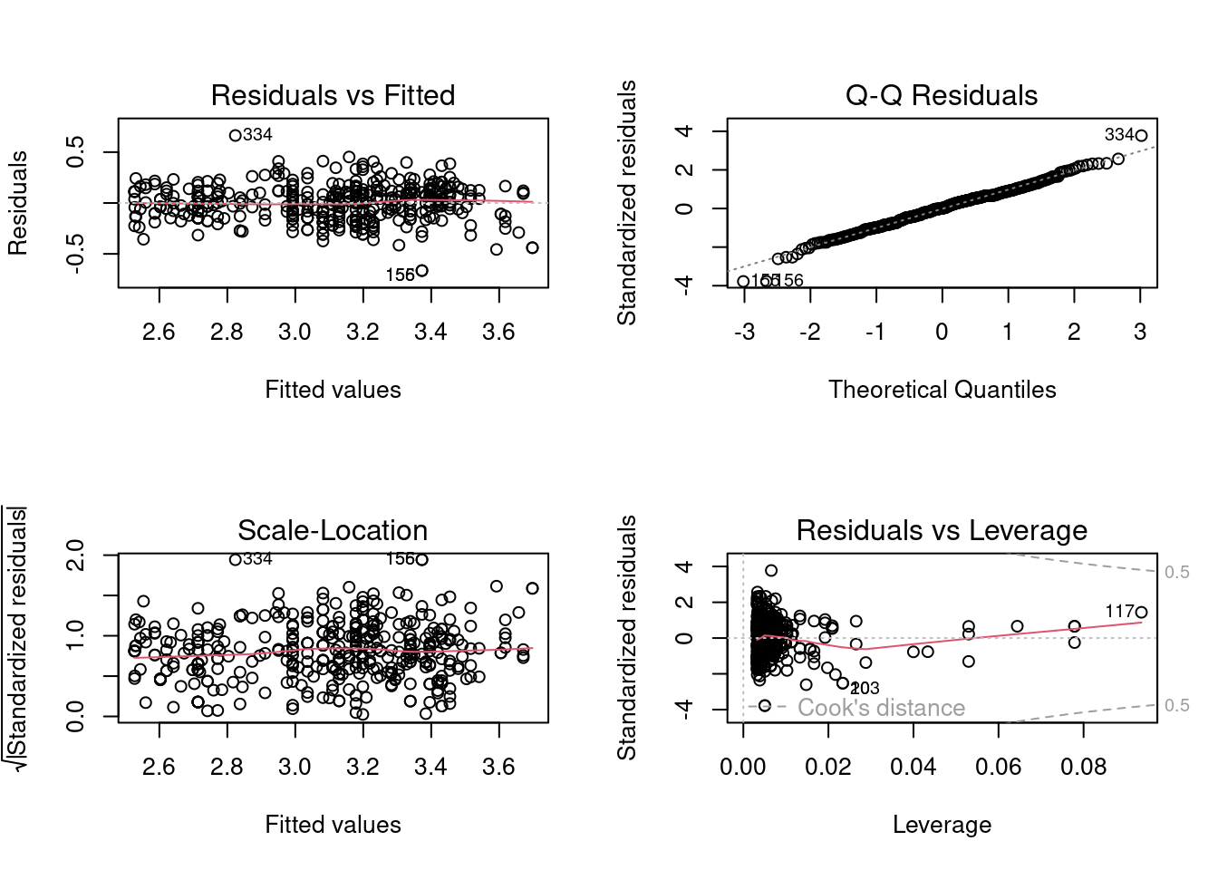
Based on the plot of residuals against fitted values, heteroscedasticity seems to be mitigated to some extent. Let us confirm with the statistical test.
bptest(log_model)
    studentized Breusch-Pagan test

data:  log_model
BP = 5.2023, df = 2, p-value = 0.07419
Assuming a significance level of \(5\%\), we do not reject the null hypothesis that the error variance is constant. Thus, the homoscedasticity assumption holds on the log transformed model.
The linear relationship assumptions seems to be satisfied. Let us check it via the \(F\) lack of fit test.
log_full_model <- lm(log(mpg)~as.factor(horsepower), data = auto_data)
anova(log_model, log_full_model)
Analysis of Variance Table
Model 1: log(mpg) ~ horsepower + I(horsepower^2)
Model 2: log(mpg) ~ as.factor(horsepower)
Res.Df RSS Df Sum of Sq F Pr(>F)
1 389 12.100
2 299 7.586 90 4.5138 1.9768 1.032e-05 ***
---
Signif. codes: 0 '***' 0.001 '**' 0.01 '*' 0.05 '.' 0.1 ' ' 1Although the \(p\)-value is higher than both the previous models indicating that the departure from linear relationship has been reduced, the model fails the \(F\) lack of fit test. However, from the residual plot, there didn’t seem to be a strong departure from the linear relationship assumption. The failure in the statistical test may be due to the presence of outliers in the data. Let us visualize the model full model along with the
colors <- c("Full log model" = "red", "Log linear model" = "blue")

ggplot(data = auto_data, aes(x = horsepower, y = log(mpg)))+
  geom_point(col = "orange")+
  geom_line(aes(y = log_full_model$fitted.values, color = "Full log model"))+
  geom_line(aes(y = log_model$fitted.values, color = "Log linear model"))+
    scale_color_manual(values = colors)+
  theme(legend.title = element_blank(),
        legend.position = c(0.85,0.9))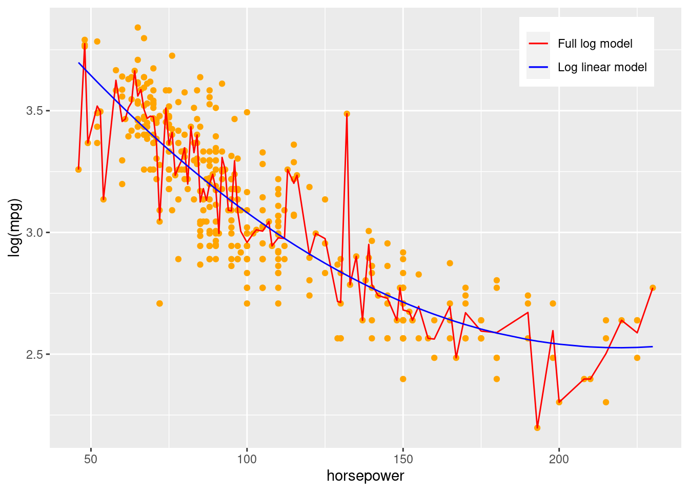
We observe that the full log model seems to be effected by outlying observations and explaining some of the noise. With the addition of more replicates at the \(X\) values corresponding to the outlying observations, the model may have passed the \(F\) lack of fit test. Thus, in this case, it appears that the relationship is indeed linear, but the failure in the statistical test is due to the full model over-fitting the data and explaining some noise as well. Another option is to bin the horsepower variable such that each bin has several replicates, and then do the \(F\) lack of fit test.
From the QQ plot, it appears that the error distribution is normal, except for three outlying values. Let us confirm the same from the normality test.
shapiro.test(log_model$residuals)
    Shapiro-Wilk normality test

data:  log_model$residuals
W = 0.99154, p-value = 0.02458
The \(p\)-value is high supporting the claim that the model satisfies the assumption of normality of error terms. The \(p\)-value would probably be higher if it was not for those three outlying points. The next step could be to analyze those three points to figure out the reason they are outlying values. For example, those three points may correspond to a particular car model that has only three observations in the data.
4.7 Box-Cox transformation
Sometimes it may be difficult to determine the appropriate transformation from diagnostic plots to correct the skewness of the error terms, unequal error variances, and non-linearity of the error function. The Box-Cox procedure automatically identifies a transformation from the family of power transformations on \(Y\). The family of power transformations is of the form:
\(Y' = Y^{\lambda}\)
The normal error regression model with the response variable a member of the family of power transformations becomes:
\(Y_i^{\lambda} = \beta_0 + \beta_1X_i\)
The Box-Cox procedure uses the method of Maximum likelihood to estimate \(\lambda\), as well as other parameters \(\beta_0, \beta_1\), and \(\sigma^2\).
Let us use the Box-Cox procedure to identify the appropriate transformation for the linear_model.
boxcox(linear_model)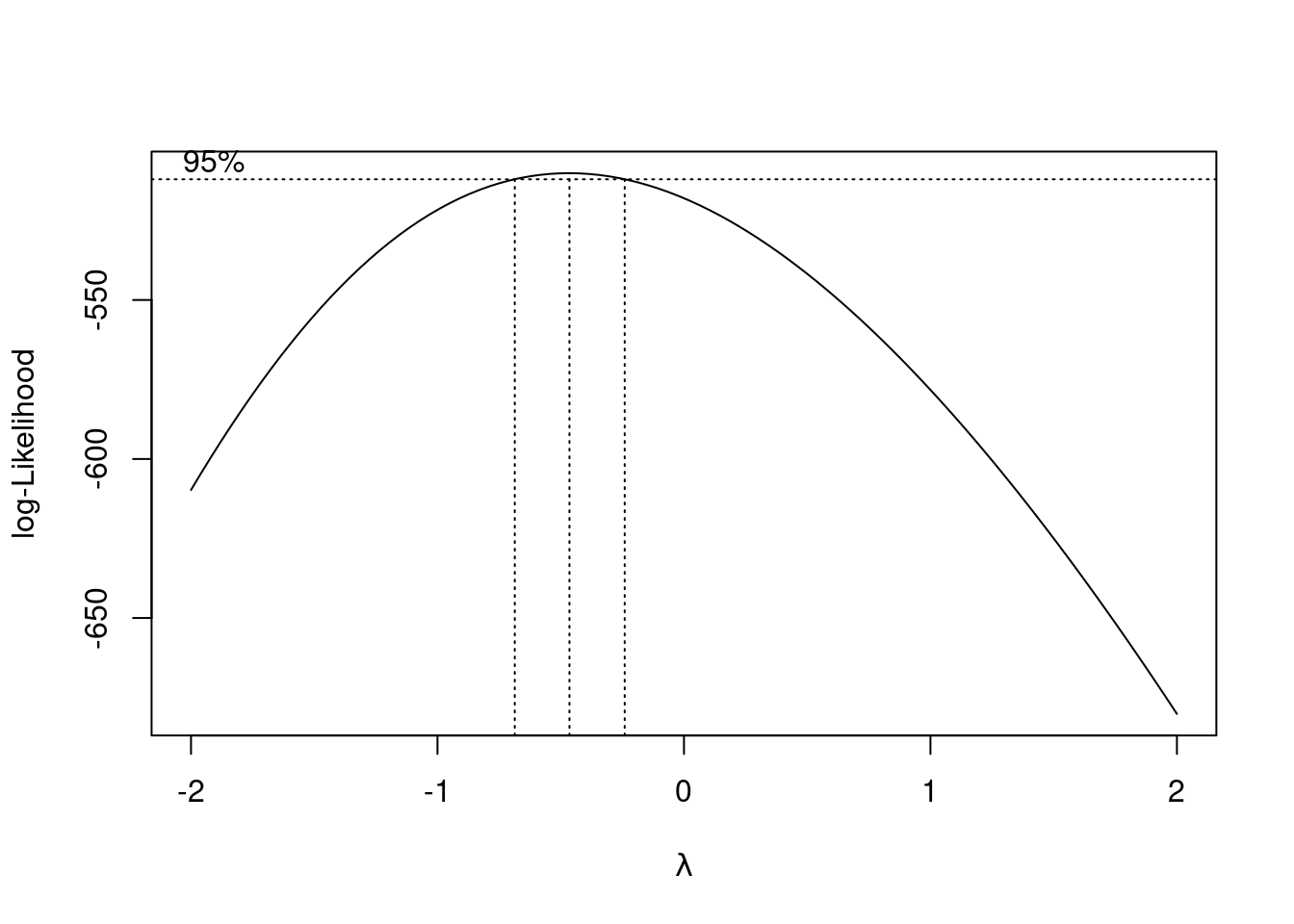
A plot of the log-likelihood vs \(\lambda\) is returned with a confidence interval for the optimal value of \(\lambda\). We can zoom-in the plot to identify the appropriate value of \(\lambda\) where the log-likelihood maximizes.
boxcox(linear_model, lambda = seq(-1, 0, 0.1))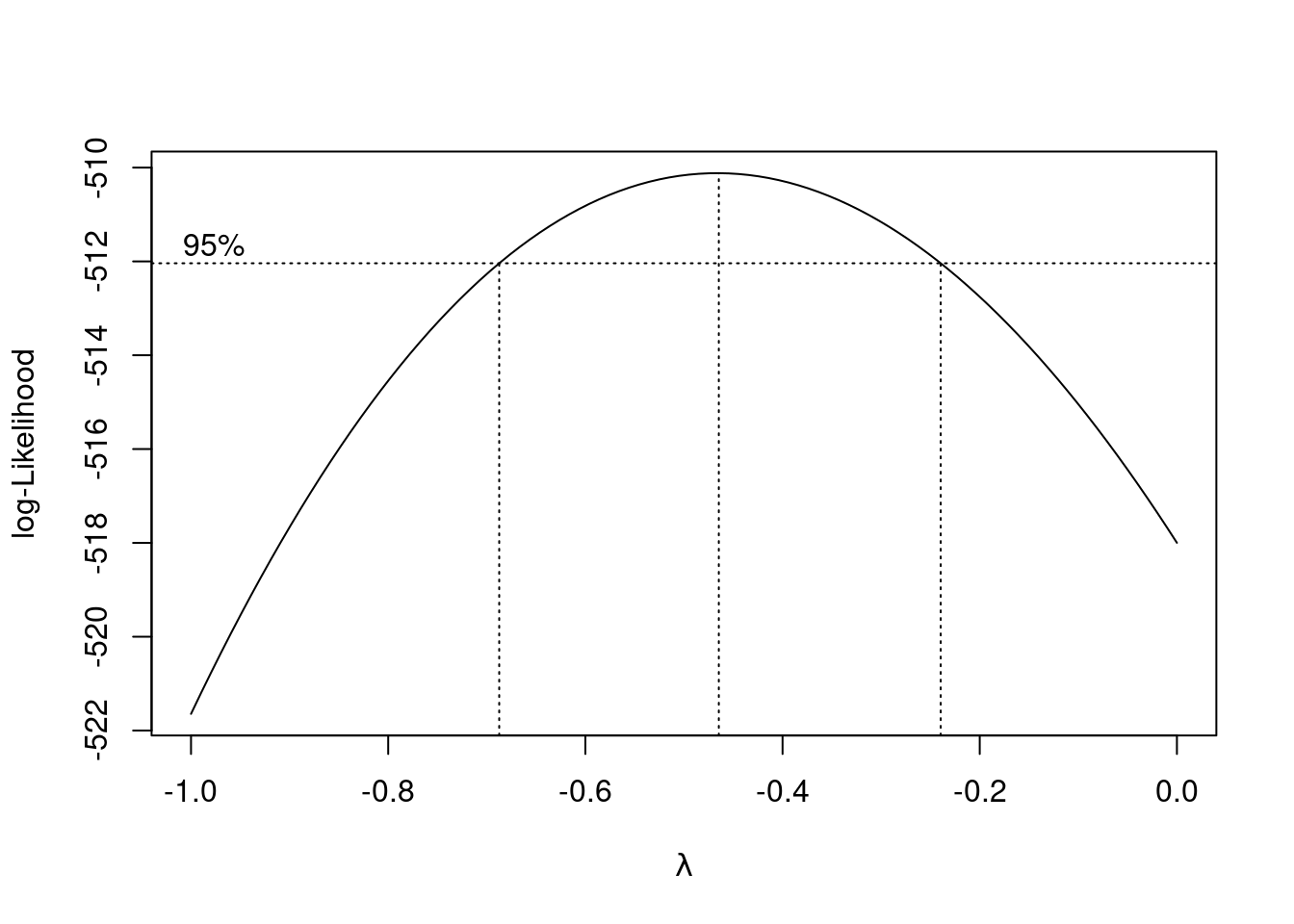
A value of \(\lambda = -0.5\) seems appropriate. Note that the log-likelihood is based on a sample. Thus, typically we don’t select the exact value of \(\lambda\) where the log-likeliood maximizes, but any value that is easier to interpret within the confidence interval. Let us consider \(\lambda = -0.5\) in this case.
boxcox_model <- lm(mpg^-0.5~horsepower, data = auto_data)
par(mfrow=c(2,2))
plot(boxcox_model)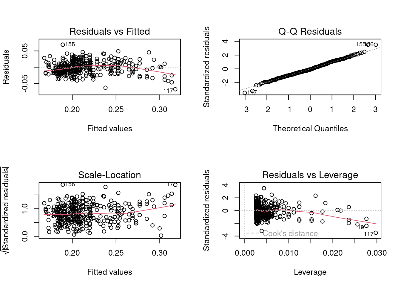
Based on the plots, the model seems to satisfy the normality of errors and homoscedasticity assumption, but there appears to be a quadratic relationship between the response and the predictor. Let us confirm our visual analysis with statistical tests.
bptest(boxcox_model)
    studentized Breusch-Pagan test

data:  boxcox_model
BP = 10.484, df = 1, p-value = 0.001204
The homoscedasticity assumption is violated, but not too severely.
shapiro.test(boxcox_model$residuals)
    Shapiro-Wilk normality test

data:  boxcox_model$residuals
W = 0.99449, p-value = 0.1721
Box-Cox transformation indeed resulted in the normal distribution of error terms.
power_full_model <- lm(mpg^-0.5~as.factor(horsepower), data = auto_data)
anova(boxcox_model, power_full_model)
Analysis of Variance Table
Model 1: mpg^-0.5 ~ horsepower
Model 2: mpg^-0.5 ~ as.factor(horsepower)
Res.Df RSS Df Sum of Sq F Pr(>F)
1 390 0.152325
2 299 0.085073 91 0.067252 2.5974 6.074e-10 ***
---
Signif. codes: 0 '***' 0.001 '**' 0.01 '*' 0.05 '.' 0.1 ' ' 1As expected based on the visual analysis, the relationship has a large departure from linearity.
Note that the Box-Cox transformation can identify the appropriate transformation for the response, but not for the predictors. Thus, we need to figure out the appropriate predictor transformation based on the diagnostic plots and/or trial and error. Let us try the quadratic transformation of the predictor \(X\) as the relationship appears to be quadratic based on the residual plot.
quadratic_boxcox_model <- lm(mpg^-0.5~horsepower+I(horsepower**2), data = auto_data)
par(mfrow = c(2,2))
plot(quadratic_boxcox_model)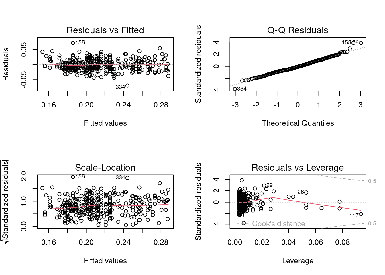
Note that the severity of the linearity assumption violation has been reduced, while the homoscedasticity and normality of errors assumptions seem to be satisfied. Note that transformation of the predictor \(X\) doesn’t change the distribution of errors. Thus, it was expected that the transformation on \(X\) will not deteriorate the model in terms of the assumptions regarding the distribution of error terms.
Let us confirm our intuition based on diagnostic plots with statistical tests.
bptest(quadratic_boxcox_model)
    studentized Breusch-Pagan test

data:  quadratic_boxcox_model
BP = 0.96746, df = 2, p-value = 0.6165
As expected, the errors are homoscedastic.
shapiro.test(quadratic_boxcox_model$residuals)
    Shapiro-Wilk normality test

data:  quadratic_boxcox_model$residuals
W = 0.98943, p-value = 0.006297
There is a slight deviation from the normal distribution, but its only due to three points as we saw earlier.
anova(quadratic_boxcox_model, power_full_model)Analysis of Variance Table
Model 1: mpg^-0.5 ~ horsepower + I(horsepower^2)
Model 2: mpg^-0.5 ~ as.factor(horsepower)
Res.Df RSS Df Sum of Sq F Pr(>F)
1 389 0.138224
2 299 0.085073 90 0.053151 2.0756 2.372e-06 ***
---
Signif. codes: 0 '***' 0.001 '**' 0.01 '*' 0.05 '.' 0.1 ' ' 1The model fails the linearity assumption test. But as noted earlier, this failure is due to the presence of very few or no replicates at some points. This potentially results in the full model explaining the noise, which in turn results in the model failing the linearity test. Again, we can bin the predictor values to have replicates for every bin, and then the model is likely to satisfy the linearity assumption.
As shown in the plot below, the full model is overfitting the data, and explaining some noise due to the absence of replicates for some values of horsepower.
ggplot(data = auto_data, aes(x = horsepower, y = mpg))+
  geom_point()+
  geom_line(aes(y = power_full_model$fitted.values^-2), color = "blue")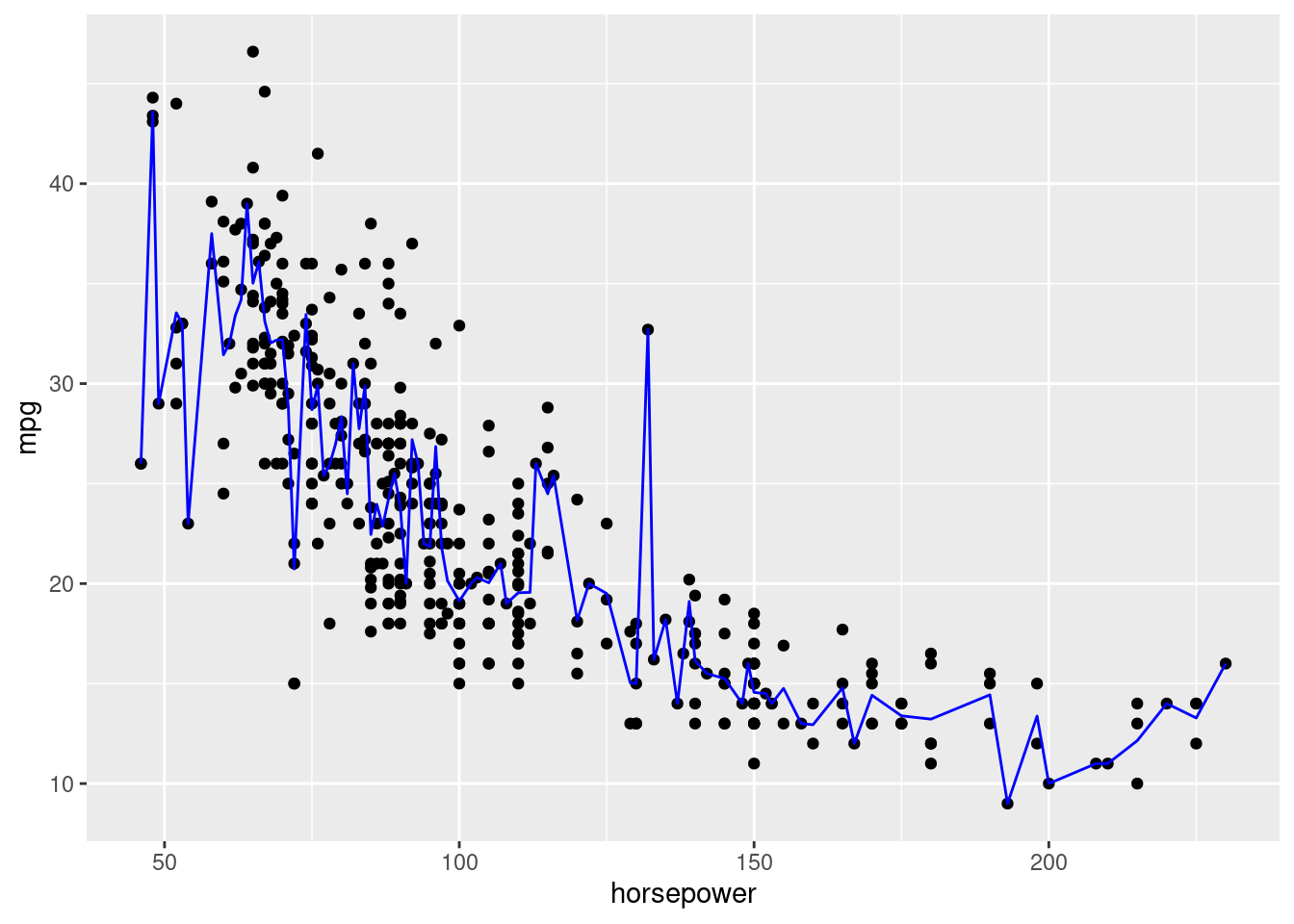
To resolve this issue, we will bin the predictor values, so that we have replicates for each distinct value of the predictor, and get a better fit for the full model
#Binning horsepower into 20 equal width bins
horsepower_bins <- cut(auto_data$horsepower, breaks = 20)
# Full model based on binned horsepower
power_full_model_binned_hp <- lm(mpg^-0.5~horsepower_bins, data = auto_data)
anova(quadratic_boxcox_model, power_full_model_binned_hp)Analysis of Variance Table
Model 1: mpg^-0.5 ~ horsepower + I(horsepower^2)
Model 2: mpg^-0.5 ~ horsepower_bins
Res.Df RSS Df Sum of Sq F Pr(>F)
1 389 0.13822
2 372 0.12912 17 0.0091085 1.5437 0.07696 .
---
Signif. codes: 0 '***' 0.001 '**' 0.01 '*' 0.05 '.' 0.1 ' ' 1Note that now the quadratic_boxcox_model model saitisfies the linearity assumption (assuming a significance level of 5%).
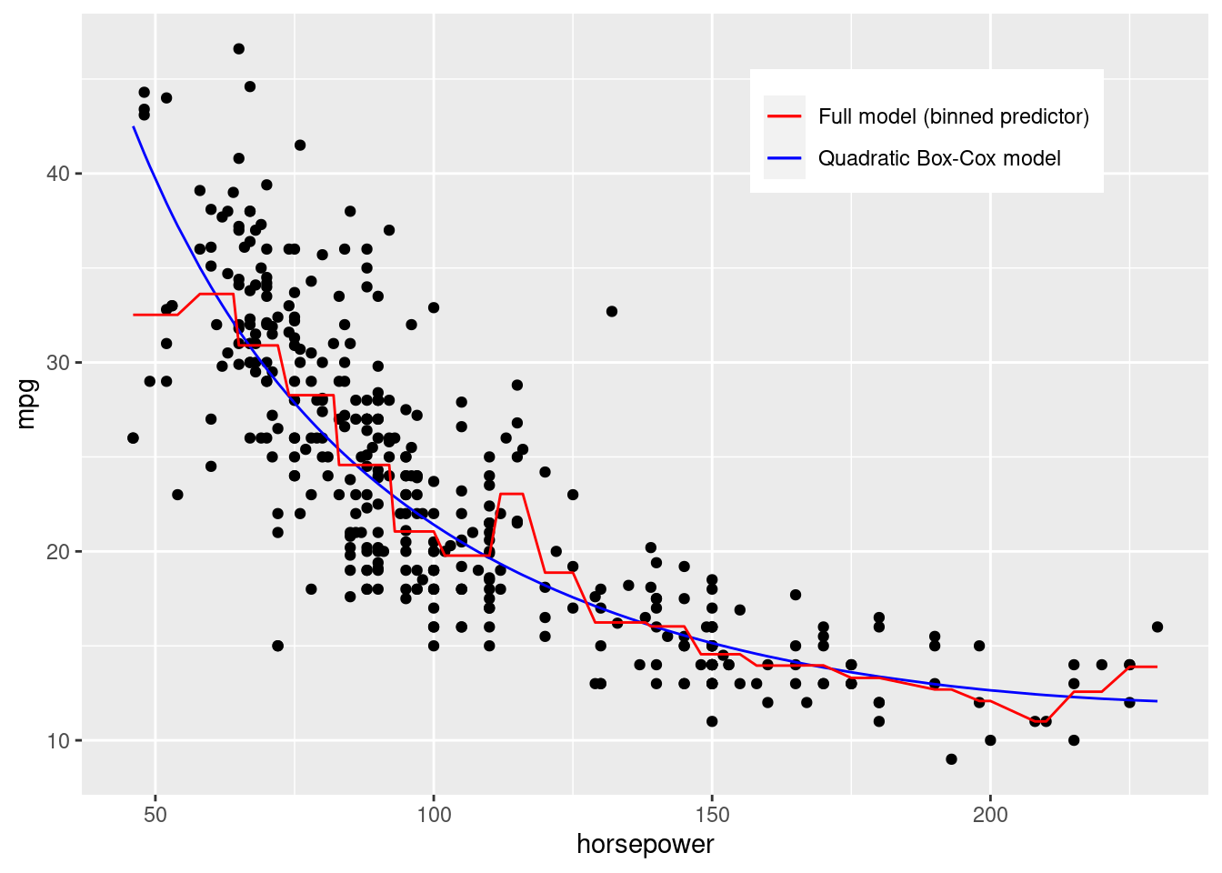
Note that our full model based on the binned horsepower values seems to better fit the data as shown in the plot below.
colors <- c("Full model (binned predictor)" = "red", "Quadratic Box-Cox model" = "blue")
ggplot(data = auto_data, aes(x = horsepower, y = mpg))+
  geom_point()+
  geom_line(aes(y = quadratic_boxcox_model$fitted.values^-2, color = "Quadratic Box-Cox model"))+
  geom_line(aes(y = power_full_model_binned_hp$fitted.values^-2, color = "Full model (binned predictor)"))+
    scale_color_manual(values = colors)+
  theme(legend.title = element_blank(),
        legend.position = c(0.75,0.85))