3  Simple linear regression model: Example

3.1 Read data

senic <- read.table('./Datasets/SENIC_data.txt')

3.2 Data pre-processing

colnames(senic) <- c("ID", "LOS", "AGE", "INFRISK", "CULT", "XRAY", "BEDS", "MEDSCHL", "REGION", "CENSUS", "NURSE", "FACS")

3.3 Model

Develop a linear regression model to Predict the length of stay based on probability of the person getting infected.

model <- lm(LOS~INFRISK, data = senic)
summary(model)

Call:
lm(formula = LOS ~ INFRISK, data = senic)

Residuals:
    Min      1Q  Median      3Q     Max 
-3.0587 -0.7776 -0.1487  0.7159  8.2805 

Coefficients:
            Estimate Std. Error t value Pr(>|t|)    
(Intercept)   6.3368     0.5213  12.156  < 2e-16 ***
INFRISK       0.7604     0.1144   6.645 1.18e-09 ***
---
Signif. codes:  0 '***' 0.001 '**' 0.01 '*' 0.05 '.' 0.1 ' ' 1

Residual standard error: 1.624 on 111 degrees of freedom
Multiple R-squared:  0.2846,    Adjusted R-squared:  0.2781 
F-statistic: 44.15 on 1 and 111 DF,  p-value: 1.177e-09

library(ggplot2)
ggplot(data = senic, aes(x = INFRISK, y = LOS))+
  geom_point()+
  geom_smooth(method = "lm")

`geom_smooth()` using formula = 'y ~ x'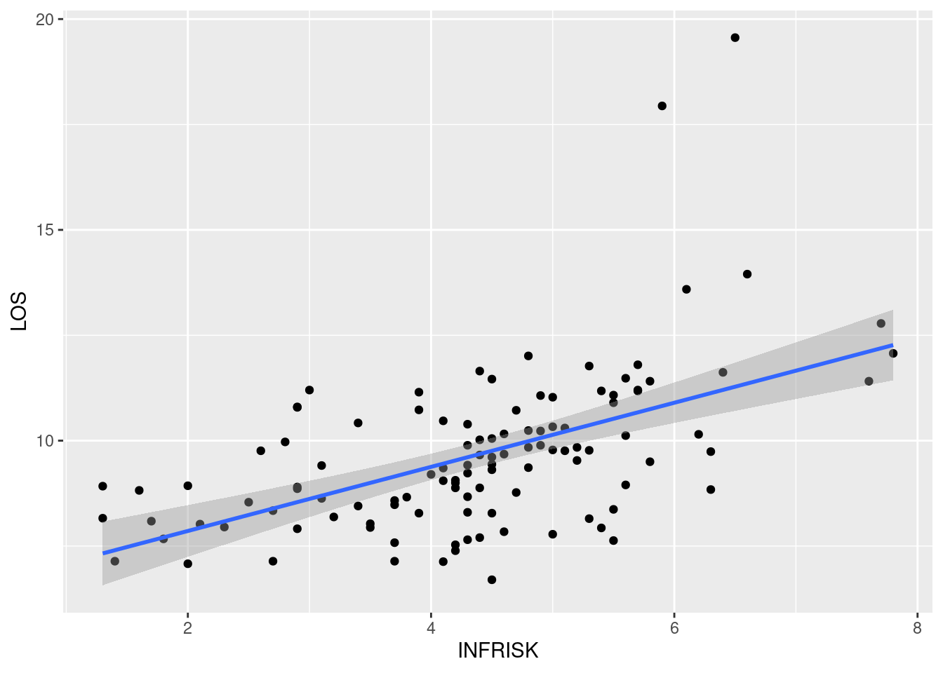

3.4 Error variance

sum(model$residuals**2)/(111)

[1] 2.637518

3.5 Confidence and Prediction intervals

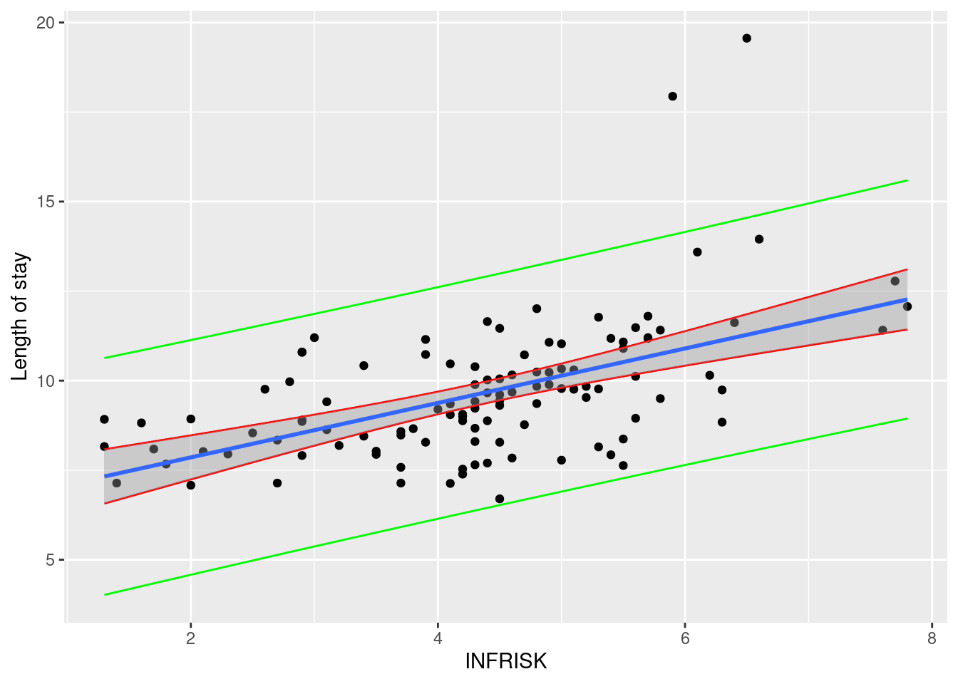
library(ggplot2)

ci <- predict(model, newdata = senic, interval = "confidence", level = 0.95)

pi <- predict(model, newdata = senic, interval = "prediction", level = 0.95)

data_ci <- cbind(senic, ci)
data_pi <- cbind(senic, pi)

ggplot(data = senic, aes(y = LOS, x = INFRISK))+
  geom_point()+
  geom_line(data = data_ci, aes(x = INFRISK, y = lwr), color = "red")+
  geom_line(data = data_ci, aes(x = INFRISK, y = upr), color = "red")+
  geom_line(data = data_pi, aes(x = INFRISK, y = lwr), color = "green")+
  geom_line(data = data_pi, aes(x = INFRISK, y = upr), color = "green")+
  geom_smooth(method = "lm")+
  labs(
    y = "Length of stay"
  )

`geom_smooth()` using formula = 'y ~ x'