8 Data wrangling

Data wrangling refers to combining, transforming, and re-arranging data to make it suitable for further analysis. We’ll use Pandas for all data wrangling operations.

import pandas as pd
import numpy as np
import seaborn as sns

8.1 Hierarchical indexing

Until now we have seen only a single level of indexing in the rows and columns of a Pandas DataFrame. Hierarchical indexing refers to having multiple index levels on an axis (row / column) of a Pandas DataFrame. It helps us to work with a higher dimensional data in a lower dimensional form.

8.1.1 Hierarchical indexing in Pandas Series

Let us define Pandas Series as we defined in Chapter 5:

#Defining a Pandas Series
series_example = pd.Series(['these','are','english','words','estas','son','palabras','en','español',
                            'ce','sont','des','françai','mots'])
series_example

0        these
1          are
2      english
3        words
4        estas
5          son
6     palabras
7           en
8      español
9           ce
10        sont
11         des
12     françai
13        mots
dtype: object

Let us use the attribute nlevels to find the number of levels of the row indices of this Series:

series_example.index.nlevels

The Series series_example has only one level of row indices.

Let us introduce another level of row indices while defining the Series:

#Defining a Pandas Series with multiple levels of row indices
series_example = pd.Series(['these','are','english','words','estas','son','palabras','en','español',
                           'ce','sont','des','françai','mots'], 
                          index=[['English']*4+['Spanish']*5+['French']*5,list(range(1,5))+list(range(1,6))*2])
series_example

English  1       these
         2         are
         3     english
         4       words
Spanish  1       estas
         2         son
         3    palabras
         4          en
         5     español
French   1          ce
         2        sont
         3         des
         4     françai
         5        mots
dtype: object

In the above Series, there are two levels of row indices:

series_example.index.nlevels

8.1.2 Hierarchical indexing in Pandas DataFrame

In a Pandas DataFrame, both the rows and the columns can have hierarchical indexing. For example, consider the DataFrame below:

data=np.array([[771517,2697000,815201,3849000],[4.2,5.6,2.8,4.6],
             [7.8,234.5,46.9,502],[6749, 597, 52, 305]])
df_example = pd.DataFrame(data,index = [['Demographics']*2+['Geography']*2,
                                      ['Population','Unemployment (%)','Area (mile-sq)','Elevation (feet)']],
                    columns = [['Illinois']*2+['California']*2,['Evanston','Chicago','San Francisco','Los Angeles']])
df_example

		Illinois		California
		Evanston	Chicago	San Francisco	Los Angeles
Demographics	Population	771517.0	2697000.0	815201.0	3849000.0
Demographics	Unemployment (%)	4.2	5.6	2.8	4.6
Geography	Area (mile-sq)	7.8	234.5	46.9	502.0
Geography	Elevation (feet)	6749.0	597.0	52.0	305.0

In the above DataFrame, both the rows and columns have 2 levels of indexing. The number of levels of column indices can be found using the attribute nlevels:

df_example.columns.nlevels

The columns attribute will now have a MultiIndex datatype in contrast to the Index datatype with single level of indexing. The same holds for row indices.

type(df_example.columns)

pandas.core.indexes.multi.MultiIndex

df_example.columns

MultiIndex([(  'Illinois',      'Evanston'),
            (  'Illinois',       'Chicago'),
            ('California', 'San Francisco'),
            ('California',   'Los Angeles')],
           )

The hierarchical levels can have names. Let us assign names to the each level of the row and column labels:

#Naming the row indices levels
df_example.index.names=['Information type', 'Statistic']

#Naming the column indices levels
df_example.columns.names=['State', 'City']

#Viewing the DataFrame
df_example

	State	Illinois		California
	City	Evanston	Chicago	San Francisco	Los Angeles
Information type	Statistic
Demographics	Population	771517.0	2697000.0	815201.0	3849000.0
Demographics	Unemployment (%)	4.2	5.6	2.8	4.6
Geography	Area (mile-sq)	7.8	234.5	46.9	502.0
Geography	Elevation (feet)	6749.0	597.0	52.0	305.0

Observe that the names of the row and column labels appear when we view the DataFrame.

8.1.2.1 `get_level_values()`

The names of the column levels can be obtained using the function get_level_values(). The outer-most level corresponds to the level = 0, and it increases as we go to the inner levels.

#Column levels at level 0 (the outer level)
df_example.columns.get_level_values(0)

Index(['Illinois', 'Illinois', 'California', 'California'], dtype='object', name='State')

#Column levels at level 1 (the inner level)
df_example.columns.get_level_values(1)

Index(['Evanston', 'Chicago', 'San Francisco', 'Los Angeles'], dtype='object', name='City')

8.1.3 Subsetting data

We can use the indices at the outer levels to concisely subset a Series / DataFrame.

The first four observations of the Series series_example correspond to the outer row index English, while the last 5 rows correspond to the outer row index Spanish. Let us subset all the observations corresponding to the outer row index English:

#Subsetting data by row-index
series_example['English']

1      these
2        are
3    english
4      words
dtype: object

Just like in the case of single level indices, if we wish to subset corresponding to multiple outer-level indices, we put the indices within an additional box bracket []. For example, let us subset all the observations corresponding to the row-indices English and French:

#Subsetting data by multiple row-indices
series_example[['English','French']]

English  1      these
         2        are
         3    english
         4      words
French   1         ce
         2       sont
         3        des
         4    françai
         5       mots
dtype: object

We can also subset data using the inner row index. However, we will need to put a : sign to indicate that the row label at the inner level is being used.

#Subsetting data by row-index
series_example[:,2]

English     are
Spanish     son
French     sont
dtype: object

#Subsetting data by multiple row-indices
series_example.loc[:,[1,2]]

English  1    these
Spanish  1    estas
French   1       ce
English  2      are
Spanish  2      son
French   2     sont
dtype: object

As in Series, we can concisely subset rows / columns in a DataFrame based on the index at the outer levels.

df_example['Illinois']

	City	Evanston	Chicago
Information type	Statistic
Demographics	Population	771517.0	2697000.0
Demographics	Unemployment (%)	4.2	5.6
Geography	Area (mile-sq)	7.8	234.5
Geography	Elevation (feet)	6749.0	597.0

Note that the dataype of each column name is a tuple. For example, let us find the datatype of the \(1^{st}\) column name:

#First column name
df_example.columns[0]

('Illinois', 'Evanston')

#Datatype of first column name
type(df_example.columns[0])

tuple

Thus columns at the inner levels can be accessed by specifying the name as a tuple. For example, let us subset the column Evanston:

#Subsetting the column 'Evanston'
df_example[('Illinois','Evanston')]

Information type  Statistic       
Demographics      Population          771517.0
                  Unemployment (%)         4.2
Geography         Area (mile-sq)           7.8
                  Elevation (feet)      6749.0
Name: (Illinois, Evanston), dtype: float64

#Subsetting the columns 'Evanston' and 'Chicago' of the outer column level 'Illinois'
df_example.loc[:,('Illinois',['Evanston','Chicago'])]

	State	Illinois
	City	Evanston	Chicago
Information type	Statistic
Demographics	Population	771517.0	2697000.0
Demographics	Unemployment (%)	4.2	5.6
Geography	Area (mile-sq)	7.8	234.5
Geography	Elevation (feet)	6749.0	597.0

8.1.4 Practice exercise 1

Read the table consisting of GDP per capita of countries from the webpage: https://en.wikipedia.org/wiki/List_of_countries_by_GDP_(nominal)_per_capita .

To only read the relevant table, read the tables that contain the word ‘Country’.

8.1.4.1

How many levels of indexing are there in the rows and columns?

dfs = pd.read_html('https://en.wikipedia.org/wiki/List_of_countries_by_GDP_(nominal)_per_capita', match = 'Country')
gdp_per_capita = dfs[0]
gdp_per_capita.head()

	Country/Territory	UN Region	IMF[4]		World Bank[5]		United Nations[6]
	Country/Territory	UN Region	Estimate	Year	Estimate	Year	Estimate	Year
0	Liechtenstein *	Europe	—	—	169049	2019	180227	2020
1	Monaco *	Europe	—	—	173688	2020	173696	2020
2	Luxembourg *	Europe	127673	2022	135683	2021	117182	2020
3	Bermuda *	Americas	—	—	110870	2021	123945	2020
4	Ireland *	Europe	102217	2022	99152	2021	86251	2020

Just by looking at the DataFrame, it seems as if there are two levels of indexing for columns and one level of indexing for rows. However, let us confirm it with the nlevels attribute.

gdp_per_capita.columns.nlevels

Yes, there are 2 levels of indexing for columns.

gdp_per_capita.index.nlevels

There is one level of indexing for rows.

8.1.4.2

Subset a DataFrame that selects the country, and the United Nations’ estimates of GDP per capita with the corresponding year.

gdp_per_capita.loc[:,['Country/Territory','United Nations[6]']]

	Country/Territory	United Nations[6]
	Country/Territory	Estimate	Year
0	Liechtenstein *	180227	2020
1	Monaco *	173696	2020
2	Luxembourg *	117182	2020
3	Bermuda *	123945	2020
4	Ireland *	86251	2020
...	...	...	...
217	Madagascar *	470	2020
218	Central African Republic *	481	2020
219	Sierra Leone *	475	2020
220	South Sudan *	1421	2020
221	Burundi *	286	2020

222 rows × 3 columns

8.1.4.3

Subset a DataFrame that selects only the World Bank and United Nations’ estimates of GDP per capita without the corresponding year or country.

gdp_per_capita.loc[:,(['World Bank[5]','United Nations[6]'],'Estimate')]

	World Bank[5]	United Nations[6]
	Estimate	Estimate
0	169049	180227
1	173688	173696
2	135683	117182
3	110870	123945
4	99152	86251
...	...	...
217	515	470
218	512	481
219	516	475
220	1120	1421
221	237	286

222 rows × 2 columns

8.1.4.4

Subset a DataFrame that selects the country and only the World Bank and United Nations’ estimates of GDP per capita without the corresponding year or country.

gdp_per_capita.loc[:,[('Country/Territory','Country/Territory'),('United Nations[6]','Estimate'),('World Bank[5]','Estimate')]]

	Country/Territory	United Nations[6]	World Bank[5]
	Country/Territory	Estimate	Estimate
0	Liechtenstein *	180227	169049
1	Monaco *	173696	173688
2	Luxembourg *	117182	135683
3	Bermuda *	123945	110870
4	Ireland *	86251	99152
...	...	...	...
217	Madagascar *	470	515
218	Central African Republic *	481	512
219	Sierra Leone *	475	516
220	South Sudan *	1421	1120
221	Burundi *	286	237

222 rows × 3 columns

8.1.4.5

Drop all columns consisting of years. Use the level argument of the drop() method.

gdp_per_capita = gdp_per_capita.drop(columns='Year',level=1)
gdp_per_capita

	Country/Territory	UN Region	IMF[4]	World Bank[5]	United Nations[6]
	Country/Territory	UN Region	Estimate	Estimate	Estimate
0	Liechtenstein *	Europe	—	169049	180227
1	Monaco *	Europe	—	173688	173696
2	Luxembourg *	Europe	127673	135683	117182
3	Bermuda *	Americas	—	110870	123945
4	Ireland *	Europe	102217	99152	86251
...	...	...	...	...	...
217	Madagascar *	Africa	522	515	470
218	Central African Republic *	Africa	496	512	481
219	Sierra Leone *	Africa	494	516	475
220	South Sudan *	Africa	328	1120	1421
221	Burundi *	Africa	293	237	286

222 rows × 5 columns

8.1.4.6

In the dataset obtained above, drop the inner level of the column labels. Use the droplevel() method.

gdp_per_capita = gdp_per_capita.droplevel(1,axis=1)
gdp_per_capita

	Country/Territory	UN Region	IMF[4]	World Bank[5]	United Nations[6]
0	Liechtenstein *	Europe	—	169049	180227
1	Monaco *	Europe	—	173688	173696
2	Luxembourg *	Europe	127673	135683	117182
3	Bermuda *	Americas	—	110870	123945
4	Ireland *	Europe	102217	99152	86251
...	...	...	...	...	...
217	Madagascar *	Africa	522	515	470
218	Central African Republic *	Africa	496	512	481
219	Sierra Leone *	Africa	494	516	475
220	South Sudan *	Africa	328	1120	1421
221	Burundi *	Africa	293	237	286

222 rows × 5 columns

8.1.5 Practice exercise 2

Recall problem 2(e) from assignment 3 on Pandas, where we needed to find the African country that is the closest to country \(G\) (Luxembourg) with regard to social indicators.

We will solve the question with the regular way in which we use single level of indexing (as you probably did during this assignment), and see if it is easier to do with hierarchical indexing.

Execute the code below that we used to pre-process data to make it suitable for answering this question.

#Pre-processing data - execute this code
social_indicator = pd.read_csv("./Datasets/social_indicator.txt",sep="\t",index_col = 0)
social_indicator.geographic_location = social_indicator.geographic_location.apply(lambda x: 'Asia' if 'Asia' in x else 'Europe' if 'Europe' in x else 'Africa' if 'Africa' in x else x)
social_indicator.rename(columns={'geographic_location':'continent'},inplace=True)
social_indicator = social_indicator.sort_index(axis=1)
social_indicator.drop(columns=['region','contraception'],inplace=True)

Below is the code to find the African country that is the closest to country \(G\) (Luxembourg) using single level of indexing. Your code in the assignment is probably similar to the one below:

#Finding the index of the country G (Luxembourg) that has the maximum GDP per capita
country_max_gdp_position = social_indicator.gdpPerCapita.argmax()

#Scaling the social indicator dataset
social_indicator_scaled = social_indicator.iloc[:,2:].apply(lambda x: (x-x.mean())/(x.std()))

#Computing the Manhattan distances of all countries from country G (Luxembourg)
manhattan_distances = (social_indicator_scaled-social_indicator_scaled.iloc[country_max_gdp_position,:]).abs().sum(axis=1)

#Finding the indices of African countries
african_countries_indices = social_indicator.loc[social_indicator.continent=='Africa',:].index

#Filtering the Manhattan distances of African countries from country G (Luxembourg)
manhattan_distances_African = manhattan_distances[african_countries_indices]

#Finding the country among African countries that has the least Manhattan distance to country G (Luxembourg)
social_indicator.loc[manhattan_distances_African.idxmin(),'country']

'Reunion'

8.1.5.1

Use the method set_index() to set continent and country as hierarchical indices of rows. Find the African country that is the closest to country \(G\) (Luxembourg) using this hierarchically indexed data. How many lines will be eliminated from the code above? Which lines will be eliminated?

Hint: Since continent and country are row indices, you don’t need to explicitly find:

The row index of country \(G\) (Luxembourg),
The row indices of African countries.
The Manhattan distances for African countries.

social_indicator.set_index(['continent','country'],inplace = True)
social_indicator_scaled = social_indicator.apply(lambda x: (x-x.mean())/(x.std()))
manhattan_distances = (social_indicator_scaled-social_indicator_scaled.loc[('Europe','Luxembourg'),:]).abs().sum(axis=1)
manhattan_distances['Africa'].idxmin()

'Reunion'

As we have converted the columns continent and country to row indices, all the lines of code where we were keeping track of the index of country \(G\), African countries, and Manhattan distances of African countries are eliminated. Three lines of code are eliminated.

Hierarchical indexing relieves us from keeping track of indices, if we set indices that are relatable to our analysis.

8.1.5.2

Use the Pandas DataFrame method mean() with the level argument to find the mean value of all social indicators for each continent.

social_indicator.mean(level=0)

	economicActivityFemale	economicActivityMale	gdpPerCapita	illiteracyFemale	illiteracyMale	infantMortality	lifeFemale	lifeMale	totalfertilityrate
continent
Asia	41.592683	79.282927	27796.390244	23.635951	13.780878	39.853659	70.724390	66.575610	3.482927
Africa	46.732258	79.445161	7127.483871	52.907226	33.673548	77.967742	56.841935	53.367742	4.889677
Oceania	51.280000	77.953333	14525.666667	9.666667	6.585200	23.666667	72.406667	67.813333	3.509333
North America	45.238095	77.166667	18609.047619	17.390286	14.609905	22.904762	75.457143	70.161905	2.804286
South America	42.008333	75.575000	15925.916667	9.991667	6.750000	34.750000	72.691667	66.975000	2.872500
Europe	52.060000	70.291429	45438.200000	2.308343	1.413543	10.571429	77.757143	70.374286	1.581714

8.1.6 Practice exercise 3

Let us try to find the areas where NU students lack in diversity. Read survey_data_clean.csv. Use hierarchical indexing to classify the columns as follows:

Classify the following variables as lifestyle:

lifestyle = ['fav_alcohol', 'parties_per_month', 'smoke', 'weed','streaming_platforms', 'minutes_ex_per_week',
       'sleep_hours_per_day', 'internet_hours_per_day', 'procrastinator', 'num_clubs','student_athlete','social_media']

Classify the following variables as personality:

personality = ['introvert_extrovert', 'left_right_brained', 'personality_type', 
       'num_insta_followers', 'fav_sport','learning_style','dominant_hand']

Classify the following variables as opinion:

opinion = ['love_first_sight', 'expected_marriage_age',  'expected_starting_salary', 'how_happy', 
       'fav_number', 'fav_letter', 'fav_season',   'political_affliation', 'cant_change_math_ability',
       'can_change_math_ability', 'math_is_genetic', 'much_effort_is_lack_of_talent']

Classify the following variables as academic information:

academic_info = ['major', 'num_majors_minors',
       'high_school_GPA', 'NU_GPA', 'school_year','AP_stats', 'used_python_before']

Classify the following variables as demographics:

demographics = [ 'only_child','birth_month', 
       'living_location_on_campus', 'age', 'height', 'height_father',
       'height_mother',  'childhood_in_US', 'gender', 'region_of_residence']

Write a function that finds the number of variables having outliers in a dataset. Apply the function to each of the 5 categories of variables in the dataset. Our hypothesis is that the category that has the maximum number of variables with outliers has the least amount of diversity. For continuous variables, use Tukey’s fences criterion to identify outliers. For categorical variables, consider levels having less than 1% observations as outliers. Assume that numeric variables that have more than 2 distinct values are continuous.

Solution:

#Using hierarchical indexing to classify columns

#Reading data
survey_data = pd.read_csv('./Datasets/survey_data_clean.csv')

#Arranging columns in the order of categories
survey_data_HI = survey_data[lifestyle+personality+opinion+academic_info+demographics]

#Creating hierarchical indexing to classify columns
survey_data_HI.columns=[['lifestyle']*len(lifestyle)+['personality']*len(personality)+['opinion']*len(opinion)+\
                       ['academic_info']*len(academic_info)+['demographics']*len(demographics),lifestyle+\
                        personality+opinion+academic_info+demographics]

#Function to identify outliers based on Tukey's fences for continous variables and 1% criterion for categorical variables
def rem_outliers(x):
    if ((len(x.value_counts())>2) & (x.dtype!='O')):#continuous variable
        q1 =x.quantile(0.25)
        q3 = x.quantile(0.75)
        intQ_range = q3-q1

        #Tukey's fences
        Lower_fence = q1 - 1.5*intQ_range
        Upper_fence = q3 + 1.5*intQ_range

        num_outliers = ((x<Lower_fence) | (x>Upper_fence)).sum()
        if num_outliers>0:
            return True
        return False
    else:                                       #categorical variable
        if np.min(x.value_counts()/len(x))<0.01:
            return True
        return False

#Number of variables containing outlier(s) in each category
for category in survey_data_HI.columns.get_level_values(0).unique():
    print("Number of missing values for category ",category," = ",survey_data_HI[category].apply(rem_outliers).sum())

Number of missing values for category  lifestyle  =  7
Number of missing values for category  personality  =  2
Number of missing values for category  opinion  =  4
Number of missing values for category  academic_info  =  3
Number of missing values for category  demographics  =  4

The lifestyle category has the highest number of variables containing outlier(s). If the hypothesis is true, then NU students have the least diversity in their lifestyle, among all the categories.

Although one may say that the lifestyle category has the the highest number of columns (as shown below), the proportion of columns having outlier(s) is also the highest for this category.

for category in survey_data_HI.columns.get_level_values(0).unique():
    print("Number of columns in category ",category," = ",survey_data_HI[category].shape[1])

Number of columns in category  lifestyle  =  12
Number of columns in category  personality  =  7
Number of columns in category  opinion  =  12
Number of columns in category  academic_info  =  7
Number of columns in category  demographics  =  10

8.1.7 Reshaping data

Apart from ease in subsetting data, hierarchical indexing also plays a role in reshaping data.

8.1.7.1 `unstack()` (Pandas Series method)

The Pandas Series method unstack() pivots the desired level of row indices to columns, thereby creating a DataFrame. By default, the inner-most level of the row labels is pivoted.

#Pivoting the inner-most Series row index to column labels
series_example_unstack = series_example.unstack()
series_example_unstack

	1	2	3	4	5
English	these	are	english	words	NaN
French	ce	sont	des	françai	mots
Spanish	estas	son	palabras	en	español

We can pivot the outer level of the row labels by specifying it in the level argument:

#Pivoting the outer row indices to column labels
series_example_unstack = series_example.unstack(level=0)
series_example_unstack

	English	French	Spanish
1	these	ce	estas
2	are	sont	son
3	english	des	palabras
4	words	françai	en
5	NaN	mots	español

8.1.7.2 `unstack()` (Pandas DataFrame method)

The Pandas DataFrame method unstack() pivots the specified level of row indices to the new inner-most level of column labels. By default, the inner-most level of the row labels is pivoted.

#Pivoting the inner level of row labels to the inner-most level of column labels
df_example.unstack()

State	Illinois								California
City	Evanston				Chicago				San Francisco				Los Angeles
Statistic	Area (mile-sq)	Elevation (feet)	Population	Unemployement (%)	Area (mile-sq)	Elevation (feet)	Population	Unemployement (%)	Area (mile-sq)	Elevation (feet)	Population	Unemployement (%)	Area (mile-sq)	Elevation (feet)	Population	Unemployement (%)
Information type
Demographics	NaN	NaN	771517.0	4.2	NaN	NaN	2697000.0	5.6	NaN	NaN	815201.0	2.8	NaN	NaN	3849000.0	4.6
Geography	7.8	6749.0	NaN	NaN	234.5	597.0	NaN	NaN	46.9	52.0	NaN	NaN	502.0	305.0	NaN	NaN

As with Series, we can pivot the outer level of the row labels by specifying it in the level argument:

#Pivoting the outer level (level = 0) of row labels to the inner-most level of column labels
df_example.unstack(level=0)

State	Illinois				California
City	Evanston		Chicago		San Francisco		Los Angeles
Information type	Demographics	Geography	Demographics	Geography	Demographics	Geography	Demographics	Geography
Statistic
Area (mile-sq)	NaN	7.8	NaN	234.5	NaN	46.9	NaN	502.0
Elevation (feet)	NaN	6749.0	NaN	597.0	NaN	52.0	NaN	305.0
Population	771517.0	NaN	2697000.0	NaN	815201.0	NaN	3849000.0	NaN
Unemployement (%)	4.2	NaN	5.6	NaN	2.8	NaN	4.6	NaN

8.1.7.3 `stack()`

The inverse of unstack() is the stack() method, which creates the inner-most level of row indices by pivoting the column labels of the prescribed level.

Note that if the column labels have only one level, we don’t need to specify a level.

#Stacking the columns of a DataFrame
series_example_unstack.stack()

English  1       these
         2         are
         3     english
         4       words
French   1          ce
         2        sont
         3         des
         4     françai
         5        mots
Spanish  1       estas
         2         son
         3    palabras
         4          en
         5     español
dtype: object

However, if the columns have multiple levels, we can specify the level to stack as the inner-most row level. By default, the inner-most column level is stacked.

#Stacking the inner-most column labels inner-most row indices
df_example.stack()

		State	California	Illinois
Information type	Statistic	City
Demographics	Population	Chicago	NaN	2697000.0
		Evanston	NaN	771517.0
		Los Angeles	3849000.0	NaN
		San Francisco	815201.0	NaN
	Unemployement (%)	Chicago	NaN	5.6
		Evanston	NaN	4.2
		Los Angeles	4.6	NaN
		San Francisco	2.8	NaN
Geography	Area (mile-sq)	Chicago	NaN	234.5
		Evanston	NaN	7.8
		Los Angeles	502.0	NaN
		San Francisco	46.9	NaN
	Elevation (feet)	Chicago	NaN	597.0
		Evanston	NaN	6749.0
		Los Angeles	305.0	NaN
		San Francisco	52.0	NaN

#Stacking the outer column labels inner-most row indices
df_example.stack(level=0)

		City	Chicago	Evanston	Los Angeles	San Francisco
Information type	Statistic	State
Demographics	Population	California	NaN	NaN	3849000.0	815201.0
	Population	Illinois	2697000.0	771517.0	NaN	NaN
	Unemployement (%)	California	NaN	NaN	4.6	2.8
	Unemployement (%)	Illinois	5.6	4.2	NaN	NaN
Geography	Area (mile-sq)	California	NaN	NaN	502.0	46.9
	Area (mile-sq)	Illinois	234.5	7.8	NaN	NaN
	Elevation (feet)	California	NaN	NaN	305.0	52.0
	Elevation (feet)	Illinois	597.0	6749.0	NaN	NaN

8.2 Merging data

The Pandas DataFrame method merge() uses columns defined as key column(s) to merge two datasets. In case the key column(s) are not defined, the overlapping column(s) are considered as the key columns.

8.2.1 Join types

When a dataset is merged with another based on key column(s), one of the following four types of join will occur depending on the repetition of the values of the key(s) in the datasets.

One-to-one, (ii) Many-to-one, (iii) One-to-Many, and (iv) Many-to-many

The type of join may sometimes determine the number of rows to be obtained in the merged dataset. If we don’t get the expected number of rows in the merged dataset, an investigation of the datsets may be neccessary to identify and resolve the issue. There may be several possible issues, for example, the dataset may not be arranged in a way that we have assumed it to be arranged.

We’ll use toy datasets to understand the above types of joins. The .csv files with the prefix student consist of the names of a few students along with their majors, and the files with the prefix skills consist of the names of majors along with the skills imparted by the respective majors.

data_student = pd.read_csv('./Datasets/student_one.csv')
data_skill = pd.read_csv('./Datasets/skills_one.csv')

8.2.1.1 One-to-one join

Each row in one dataset is linked (or related) to a single row in another dataset based on the key column(s).

data_student

	Student	Major
0	Kitana	Statistics
1	Jax	Computer Science
2	Sonya	Material Science
3	Johnny	Music

data_skill

	Major	Skills
0	Statistics	Inference
1	Computer Science	Machine learning
2	Material Science	Structure prediction
3	Music	Opera

pd.merge(data_student,data_skill)

	Student	Major	Skills
0	Kitana	Statistics	Inference
1	Jax	Computer Science	Machine learning
2	Sonya	Material Science	Structure prediction
3	Johnny	Music	Opera

8.2.1.2 Many-to-one join

One or more rows in one dataset is linked (or related) to a single row in another dataset based on the key column(s).

data_student = pd.read_csv('./Datasets/student_many.csv')
data_skill = pd.read_csv('./Datasets/skills_one.csv')

data_student

	Student	Major
0	Kitana	Statistics
1	Kitana	Computer Science
2	Jax	Computer Science
3	Sonya	Material Science
4	Johnny	Music
5	Johnny	Statistics

data_skill

	Major	Skills
0	Statistics	Inference
1	Computer Science	Machine learning
2	Material Science	Structure prediction
3	Music	Opera

pd.merge(data_student,data_skill)

	Student	Major	Skills
0	Kitana	Statistics	Inference
1	Johnny	Statistics	Inference
2	Kitana	Computer Science	Machine learning
3	Jax	Computer Science	Machine learning
4	Sonya	Material Science	Structure prediction
5	Johnny	Music	Opera

8.2.1.3 One-to-many join

Each row in one dataset is linked (or related) to one, or more rows in another dataset based on the key column(s).

data_student = pd.read_csv('./Datasets/student_one.csv')
data_skill = pd.read_csv('./Datasets/skills_many.csv')

data_student

	Student	Major
0	Kitana	Statistics
1	Jax	Computer Science
2	Sonya	Material Science
3	Johnny	Music

data_skill

	Major	Skills
0	Statistics	Inference
1	Statistics	Modeling
2	Computer Science	Machine learning
3	Computer Science	Computing
4	Material Science	Structure prediction
5	Music	Opera
6	Music	Pop
7	Music	Classical

pd.merge(data_student,data_skill)

	Student	Major	Skills
0	Kitana	Statistics	Inference
1	Kitana	Statistics	Modeling
2	Jax	Computer Science	Machine learning
3	Jax	Computer Science	Computing
4	Sonya	Material Science	Structure prediction
5	Johnny	Music	Opera
6	Johnny	Music	Pop
7	Johnny	Music	Classical

8.2.1.4 Many-to-many join

One, or more, rows in one dataset is linked (or related) to one, or more, rows in another dataset using the key column(s).

data_student = pd.read_csv('./Datasets/student_many.csv')
data_skill = pd.read_csv('./Datasets/skills_many.csv')

data_student

	Student	Major
0	Kitana	Statistics
1	Kitana	Computer Science
2	Jax	Computer Science
3	Sonya	Material Science
4	Johnny	Music
5	Johnny	Statistics

data_skill

	Major	Skills
0	Statistics	Inference
1	Statistics	Modeling
2	Computer Science	Machine learning
3	Computer Science	Computing
4	Material Science	Structure prediction
5	Music	Opera
6	Music	Pop
7	Music	Classical

pd.merge(data_student,data_skill)

	Student	Major	Skills
0	Kitana	Statistics	Inference
1	Kitana	Statistics	Modeling
2	Johnny	Statistics	Inference
3	Johnny	Statistics	Modeling
4	Kitana	Computer Science	Machine learning
5	Kitana	Computer Science	Computing
6	Jax	Computer Science	Machine learning
7	Jax	Computer Science	Computing
8	Sonya	Material Science	Structure prediction
9	Johnny	Music	Opera
10	Johnny	Music	Pop
11	Johnny	Music	Classical

Note that there are two ‘Statistics’ rows in data_student, and two ‘Statistics’ rows in data_skill, resulting in 2x2 = 4 ‘Statistics’ rows in the merged data. The same is true for the ‘Computer Science’ Major.

8.2.2 Join types with `how` argument

The above mentioned types of join (one-to-one, many-to-one, etc.) occur depening on the structure of the datasets being merged. We don’t have control over the type of join. However, we can control how the joins are occurring. We can merge (or join) two datasets in one of the following four ways:

inner join, (ii) left join, (iii) right join, (iv) outer join

8.2.2.1 inner join

This is the join that occurs by default, i.e., without specifying the how argument in the merge() function. In inner join, only those observations are merged that have the same value(s) in the key column(s) of both the datasets.

data_student = pd.read_csv('./Datasets/student_how.csv')
data_skill = pd.read_csv('./Datasets/skills_how.csv')

data_student

	Student	Major
0	Kitana	Statistics
1	Jax	Computer Science
2	Sonya	Material Science

data_skill

	Major	Skills
0	Statistics	Inference
1	Computer Science	Machine learning
2	Music	Opera

pd.merge(data_student,data_skill)

	Student	Major	Skills
0	Kitana	Statistics	Inference
1	Jax	Computer Science	Machine learning

When you may use inner join? You should use inner join when you cannot carry out the analysis unless the observation corresponding to the key column(s) is present in both the tables.

Example: Suppose you wish to analyze the association between vaccinations and covid infection rate based on country-level data. In one of the datasets, you have the infection rate for each country, while in the other one you have the number of vaccinations in each country. The countries which have either the vaccination or the infection rate missing, cannot help analyze the association. In such as case you may be interested only in countries that have values for both the variables. Thus, you will use inner join to discard the countries with either value missing.

8.2.2.2 left join

In left join, the merged dataset will have all the rows of the dataset that is specified first in the merge() function. Only those observations of the other dataset will be merged whose value(s) in the key column(s) exist in the dataset specified first in the merge() function.

pd.merge(data_student,data_skill,how='left')

	Student	Major	Skills
0	Kitana	Statistics	Inference
1	Jax	Computer Science	Machine learning
2	Sonya	Material Science	NaN

When you may use left join? You should use left join when the primary variable(s) of interest are present in the one of the datasets, and whose missing values cannot be imputed. The variable(s) in the other dataset may not be as important or it may be possible to reasonably impute their values, if missing corresponding to the observation in the primary dataset.

Examples:

Suppose you wish to analyze the association between the covid infection rate and the government effectiveness score (a metric used to determine the effectiveness of the government in implementing policies, upholding law and order etc.) based on the data of all countries. Let us say that one of the datasets contains the covid infection rate, while the other one contains the government effectiveness score for each country. If the infection rate for a country is missing, it might be hard to impute. However, the government effectiveness score may be easier to impute based on GDP per capita, crime rate etc. - information that is easily available online. In such a case, you may wish to use a left join where you keep all the countries for which the infection rate is known.
Suppose you wish to analyze the association between demographics such as age, income etc. and the amount of credit card spend. Let us say one of the datasets contains the demographic information of each customer, while the other one contains the credit card spend for the customers who made at least one purchase. In such as case, you may want to do a left join as customers not making any purchase might be absent in the card spend data. Their spend can be imputed as zero after merging the datasets.

8.2.2.3 right join

In right join, the merged dataset will have all the rows of the dataset that is specified second in the merge() function. Only those observations of the other dataset will be merged whose value(s) in the key column(s) exist in the dataset specified second in the merge() function.

pd.merge(data_student,data_skill,how='right')

	Student	Major	Skills
0	Kitana	Statistics	Inference
1	Jax	Computer Science	Machine learning
2	NaN	Music	Opera

When you may use right join? You can always use a left join instead of a right join. Their purpose is the same.

8.2.2.4 outer join

In outer join, the merged dataset will have all the rows of both the datasets being merged.

pd.merge(data_student,data_skill,how='outer')

	Student	Major	Skills
0	Kitana	Statistics	Inference
1	Jax	Computer Science	Machine learning
2	Sonya	Material Science	NaN
3	NaN	Music	Opera

When you may use outer join? You should use an outer join when you cannot afford to lose data present in either of the tables. All the other joins may result in loss of data.

Example: Suppose I took two course surveys for this course. If I need to analyze student sentiment during the course, I will take an outer join of both the surveys. Assume that each survey is a dataset, where each row corresponds to a unique student. Even if a student has answered one of the two surverys, it will be indicative of the sentiment, and will be useful to keep in the merged dataset.

8.3 Concatenating datasets

The Pandas DataFrame method concat() is used to stack datasets along an axis. The method is similar to NumPy’s concatenate() method.

Example: You are given the life expectancy data of each continent as a separate *.csv file. Visualize the change of life expectancy over time for different continents.

data_asia = pd.read_csv('./Datasets/gdp_lifeExpec_Asia.csv')
data_europe = pd.read_csv('./Datasets/gdp_lifeExpec_Europe.csv')
data_africa = pd.read_csv('./Datasets/gdp_lifeExpec_Africa.csv')
data_oceania = pd.read_csv('./Datasets/gdp_lifeExpec_Oceania.csv')
data_americas = pd.read_csv('./Datasets/gdp_lifeExpec_Americas.csv')

#Appending all the data files, i.e., stacking them on top of each other
data_all_continents = pd.concat([data_asia,data_europe,data_africa,data_oceania,data_americas],keys = ['Asia','Europe','Africa','Oceania','Americas'])
data_all_continents

		country	year	lifeExp	pop	gdpPercap
Asia	0	Afghanistan	1952	28.801	8425333	779.445314
	1	Afghanistan	1957	30.332	9240934	820.853030
	2	Afghanistan	1962	31.997	10267083	853.100710
	3	Afghanistan	1967	34.020	11537966	836.197138
	4	Afghanistan	1972	36.088	13079460	739.981106
...	...	...	...	...	...	...
Americas	295	Venezuela	1987	70.190	17910182	9883.584648
	296	Venezuela	1992	71.150	20265563	10733.926310
	297	Venezuela	1997	72.146	22374398	10165.495180
	298	Venezuela	2002	72.766	24287670	8605.047831
	299	Venezuela	2007	73.747	26084662	11415.805690

1704 rows × 5 columns

Let’s have the continent as a column as we need to use that in the visualization.

data_all_continents.reset_index(inplace = True)

data_all_continents.head()

	level_0	level_1	country	year	lifeExp	pop	gdpPercap
0	Asia	0	Afghanistan	1952	28.801	8425333	779.445314
1	Asia	1	Afghanistan	1957	30.332	9240934	820.853030
2	Asia	2	Afghanistan	1962	31.997	10267083	853.100710
3	Asia	3	Afghanistan	1967	34.020	11537966	836.197138
4	Asia	4	Afghanistan	1972	36.088	13079460	739.981106

data_all_continents.drop(columns = 'level_1',inplace = True)
data_all_continents.rename(columns = {'level_0':'continent'},inplace = True)
data_all_continents.head()

	continent	country	year	lifeExp	pop	gdpPercap
0	Asia	Afghanistan	1952	28.801	8425333	779.445314
1	Asia	Afghanistan	1957	30.332	9240934	820.853030
2	Asia	Afghanistan	1962	31.997	10267083	853.100710
3	Asia	Afghanistan	1967	34.020	11537966	836.197138
4	Asia	Afghanistan	1972	36.088	13079460	739.981106

#change of life expectancy over time for different continents
a = sns.FacetGrid(data_all_continents,col = 'continent',col_wrap = 3,height = 4.5,aspect = 1)#height = 3,aspect = 0.8)
a.map(sns.lineplot,'year','lifeExp')
a.add_legend()

In the above example, datasets were appended (or stacked on top of each other).

Datasets can also be concatenated side-by-side (by providing the argument axis = 1 with the concat() function) as we saw with the merge function.

8.3.1 Practice exercise 4

Read the documentations of the Pandas DataFrame methods merge() and concat(), and identify the differences. Mention examples when you can use (i) either, (ii) only concat(), (iii) only merge()

Solution:

If we need to merge datasets using row indices, we can use either function.
If we need to stack datasets one on top of the other, we can only use concat()
If we need to merge datasets using overlapping columns we can only use merge()

8.4 Reshaping data

Data often needs to be re-arranged to ease analysis.

8.4.1 Pivoting “long” to “wide” format

`pivot()`

This function helps re-arrange data from the ‘long’ form to a ‘wide’ form.

Example: Let us consider the dataset data_all_continents obtained in the previous section after concatenating the data of all the continents.

data_all_continents.head()

	continent	country	year	lifeExp	pop	gdpPercap
0	Asia	Afghanistan	1952	28.801	8425333	779.445314
1	Asia	Afghanistan	1957	30.332	9240934	820.853030
2	Asia	Afghanistan	1962	31.997	10267083	853.100710
3	Asia	Afghanistan	1967	34.020	11537966	836.197138
4	Asia	Afghanistan	1972	36.088	13079460	739.981106

8.4.1.1 Pivoting a single column

For visualizing life expectancy in 2007 against life expectancy in 1957, we will need to filter the data, and then make the plot. Everytime that we need to compare a metric for a year against another year, we will need to filter the data.

If we need to often compare metrics of a year against another year, it will be easier to have each year as a separate column, instead of having all years in a single column.

As we are increasing the number of columns and decreasing the number of rows, we are re-arranging the data from long-form to wide-form.

data_wide = data_all_continents.pivot(index = ['continent','country'],columns = 'year',values = 'lifeExp')

data_wide.head()

	year	1952	1957	1962	1967	1972	1977	1982	1987	1992	1997	2002	2007
continent	country
Africa	Algeria	43.077	45.685	48.303	51.407	54.518	58.014	61.368	65.799	67.744	69.152	70.994	72.301
	Angola	30.015	31.999	34.000	35.985	37.928	39.483	39.942	39.906	40.647	40.963	41.003	42.731
	Benin	38.223	40.358	42.618	44.885	47.014	49.190	50.904	52.337	53.919	54.777	54.406	56.728
	Botswana	47.622	49.618	51.520	53.298	56.024	59.319	61.484	63.622	62.745	52.556	46.634	50.728
	Burkina Faso	31.975	34.906	37.814	40.697	43.591	46.137	48.122	49.557	50.260	50.324	50.650	52.295

With values of year as columns, it is easy to compare any metric for different years.

#visualizing the change in life expectancy of all countries in 2007 as compared to that in 1957, i.e., the overall change in life expectancy in 50 years. 
sns.scatterplot(data = data_wide, x = 1957,y=2007,hue = 'continent')
sns.lineplot(data = data_wide, x = 1957,y = 1957)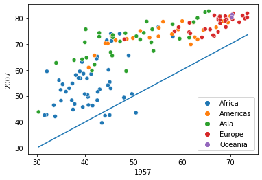

Observe that for some African countries, the life expectancy has decreased after 50 years. It is worth investigating these countries to identify factors associated with the decrease.

8.4.1.2 Pivoting multiple columns

In the above transformation, we retained only lifeExp in the ‘wide’ dataset. Suppose, we are also interested in visualizing GDP per capita of countries in one year against another year. In that case, we must have gdpPercap in the ’wide’-form data as well.

Let us create a dataset named as data_wide_lifeExp_gdpPercap that will contain both lifeExp and gdpPercap for each year in a separate column. We will specify the columns to pivot in the values argument of the pivot() function.

data_wide_lifeExp_gdpPercap = data_all_continents.pivot(index = ['continent','country'],columns = 'year',values = ['lifeExp','gdpPercap'])
data_wide_lifeExp_gdpPercap.head()

		lifeExp										...	gdpPercap
	year	1952	1957	1962	1967	1972	1977	1982	1987	1992	1997	...	1962	1967	1972	1977	1982	1987	1992	1997	2002	2007
continent	country
Africa	Algeria	43.077	45.685	48.303	51.407	54.518	58.014	61.368	65.799	67.744	69.152	...	2550.816880	3246.991771	4182.663766	4910.416756	5745.160213	5681.358539	5023.216647	4797.295051	5288.040382	6223.367465
	Angola	30.015	31.999	34.000	35.985	37.928	39.483	39.942	39.906	40.647	40.963	...	4269.276742	5522.776375	5473.288005	3008.647355	2756.953672	2430.208311	2627.845685	2277.140884	2773.287312	4797.231267
	Benin	38.223	40.358	42.618	44.885	47.014	49.190	50.904	52.337	53.919	54.777	...	949.499064	1035.831411	1085.796879	1029.161251	1277.897616	1225.856010	1191.207681	1232.975292	1372.877931	1441.284873
	Botswana	47.622	49.618	51.520	53.298	56.024	59.319	61.484	63.622	62.745	52.556	...	983.653976	1214.709294	2263.611114	3214.857818	4551.142150	6205.883850	7954.111645	8647.142313	11003.605080	12569.851770
	Burkina Faso	31.975	34.906	37.814	40.697	43.591	46.137	48.122	49.557	50.260	50.324	...	722.512021	794.826560	854.735976	743.387037	807.198586	912.063142	931.752773	946.294962	1037.645221	1217.032994

5 rows × 24 columns

The metric for each year is now in a separate column, and can be visualized directly. Note that re-arranging the dataset from the ‘long’-form to ‘wide-form’ leads to hierarchical indexing of columns when multiple ‘values’ need to be re-arranged. In this case, the multiple ‘values’ that need to be re-arranged are lifeExp and gdpPercap.

8.4.2 Melting “wide” to “long” format

`melt()`

This function is used to re-arrange the dataset from the ‘wide’ form to the ‘long’ form.

8.4.2.1 Melting columns with a single type of value

Let us consider data_wide created in the previous section.

data_wide.head()

	year	1952	1957	1962	1967	1972	1977	1982	1987	1992	1997	2002	2007
continent	country
Africa	Algeria	43.077	45.685	48.303	51.407	54.518	58.014	61.368	65.799	67.744	69.152	70.994	72.301
	Angola	30.015	31.999	34.000	35.985	37.928	39.483	39.942	39.906	40.647	40.963	41.003	42.731
	Benin	38.223	40.358	42.618	44.885	47.014	49.190	50.904	52.337	53.919	54.777	54.406	56.728
	Botswana	47.622	49.618	51.520	53.298	56.024	59.319	61.484	63.622	62.745	52.556	46.634	50.728
	Burkina Faso	31.975	34.906	37.814	40.697	43.591	46.137	48.122	49.557	50.260	50.324	50.650	52.295

Suppose, we wish to visualize the change of life expectancy over time for different continents, as we did in section 8.3. For plotting lifeExp against year, all the years must be in a single column. Thus, we need to melt the columns of data_wide to a single column and call it year.

But before melting the columns in the above dataset, we will convert continent to a column, as we need to make subplots based on continent.

The Pandas DataFrame method reset_index() can be used to remove one or more levels of indexing from the DataFrame.

#Making 'continent' a column instead of row-index at level 0
data_wide.reset_index(inplace=True,level=0)
data_wide.head()

year	continent	1952	1957	1962	1967	1972	1977	1982	1987	1992	1997	2002	2007
country
Algeria	Africa	43.077	45.685	48.303	51.407	54.518	58.014	61.368	65.799	67.744	69.152	70.994	72.301
Angola	Africa	30.015	31.999	34.000	35.985	37.928	39.483	39.942	39.906	40.647	40.963	41.003	42.731
Benin	Africa	38.223	40.358	42.618	44.885	47.014	49.190	50.904	52.337	53.919	54.777	54.406	56.728
Botswana	Africa	47.622	49.618	51.520	53.298	56.024	59.319	61.484	63.622	62.745	52.556	46.634	50.728
Burkina Faso	Africa	31.975	34.906	37.814	40.697	43.591	46.137	48.122	49.557	50.260	50.324	50.650	52.295

data_melted=pd.melt(data_wide,id_vars = ['continent'],var_name = 'Year',value_name = 'LifeExp')
data_melted.head()

	continent	Year	LifeExp
0	Africa	1952	43.077
1	Africa	1952	30.015
2	Africa	1952	38.223
3	Africa	1952	47.622
4	Africa	1952	31.975

With the above DataFrame, we can visualize the mean life expectancy against year separately for each continent.

If we wish to have country also in the above data, we can keep it while resetting the index:

#Creating 'data_wide' again
data_wide = data_all_continents.pivot(index = ['continent','country'],columns = 'year',values = 'lifeExp')

#Resetting the row-indices to default values
data_wide.reset_index(inplace=True)
data_wide.head()

year	continent	country	1952	1957	1962	1967	1972	1977	1982	1987	1992	1997	2002	2007
0	Africa	Algeria	43.077	45.685	48.303	51.407	54.518	58.014	61.368	65.799	67.744	69.152	70.994	72.301
1	Africa	Angola	30.015	31.999	34.000	35.985	37.928	39.483	39.942	39.906	40.647	40.963	41.003	42.731
2	Africa	Benin	38.223	40.358	42.618	44.885	47.014	49.190	50.904	52.337	53.919	54.777	54.406	56.728
3	Africa	Botswana	47.622	49.618	51.520	53.298	56.024	59.319	61.484	63.622	62.745	52.556	46.634	50.728
4	Africa	Burkina Faso	31.975	34.906	37.814	40.697	43.591	46.137	48.122	49.557	50.260	50.324	50.650	52.295

#Melting the 'year' column
data_melted=pd.melt(data_wide,id_vars = ['continent','country'],var_name = 'Year',value_name = 'LifeExp')
data_melted.head()

	continent	country	Year	LifeExp
0	Africa	Algeria	1952	43.077
1	Africa	Angola	1952	30.015
2	Africa	Benin	1952	38.223
3	Africa	Botswana	1952	47.622
4	Africa	Burkina Faso	1952	31.975

8.4.2.2 Melting columns with multiple types of values

Consider the dataset created in Section 8.4.1.2. It has two types of values - lifeExp and gdpPercapita, which are the column labels at the outer level. The melt() function will melt all the years of data into a single column. However, it will create another column based on the outer level column labels - lifeExp and gdpPercapita to distinguish between these two types of values. Here, we see that the function melt() internally uses hierarchical indexing to handle the transformation of multiple types of columns.

data_melt = pd.melt(data_wide_lifeExp_gdpPercap.reset_index(),id_vars = ['continent','country'],var_name = ['Metric','year'])
data_melt.head()

	continent	country	Metric	year	value
0	Africa	Algeria	lifeExp	1952	43.077
1	Africa	Angola	lifeExp	1952	30.015
2	Africa	Benin	lifeExp	1952	38.223
3	Africa	Botswana	lifeExp	1952	47.622
4	Africa	Burkina Faso	lifeExp	1952	31.975

Although the data above is in ‘long’-form, it is not quiet in its original format, as in data_all_continents. We need to pivot again by Metric to have two separate columns of gdpPercap and lifeExp.

data_restore = data_melt.pivot(index = ['continent','country','year'],columns = 'Metric')
data_restore.head()

			value
		Metric	gdpPercap	lifeExp
continent	country	year
Africa	Algeria	1952	2449.008185	43.077
		1957	3013.976023	45.685
		1962	2550.816880	48.303
		1967	3246.991771	51.407
		1972	4182.663766	54.518

Now, we can convert the row indices of continent and country to columns to restore the dataset to the same form as data_all_continents.

data_restore.reset_index(inplace = True)
data_restore.head()

	continent	country	year	value
Metric				gdpPercap	lifeExp
0	Africa	Algeria	1952	2449.008185	43.077
1	Africa	Algeria	1957	3013.976023	45.685
2	Africa	Algeria	1962	2550.816880	48.303
3	Africa	Algeria	1967	3246.991771	51.407
4	Africa	Algeria	1972	4182.663766	54.518

8.4.3 Practice exercise 5

8.4.3.1

Both unstack() and pivot() seem to transform the data from the ‘long’ form to the ‘wide’ form. Is there a difference between the two functions?

Solution:

Yes, both the functions transform the data from the ‘long’ form to the ‘wide’ form. However, unstack() pivots the row indices, while pivot() pivots the columns of the DataFrame.

Even though both functions are a bit different, it is possible to just use one of them to perform a reshaping operation. If we wish to pivot a column, we can either use pivot() directly on the column, or we can convert the column to row indices and then use unstack(). If we wish to pivot row indices, we can either use unstack() directly on the row indices, or we can convert row indices to a column and then use pivot().

To summarise, using one function may be more straightforward than using the other one, but either can be used for reshaping data from the ‘long’ form to the ‘wide’ form.

Below is an example where we perform the same reshaping operation with either function.

Consider the data data_all_continent. Suppose we wish to transform it to data_wide as we did using pivot() in Section 8.4.1.1. Let us do it using unstack(), instead of pivot().

The first step will be to reindex data to set year as row indices, and also continent and country as row indices because these two column were set as indices with the pivot() function in Section 8.4.1.1.

#Reindexing data to make 'continent', 'country', and 'year' as hierarchical row indices
data_reindexed=data_all_continents.set_index(['continent','country','year'])
data_reindexed

			lifeExp	pop	gdpPercap
continent	country	year
Asia	Afghanistan	1952	28.801	8425333	779.445314
		1957	30.332	9240934	820.853030
		1962	31.997	10267083	853.100710
		1967	34.020	11537966	836.197138
		1972	36.088	13079460	739.981106
...	...	...	...	...	...
Americas	Venezuela	1987	70.190	17910182	9883.584648
		1992	71.150	20265563	10733.926310
		1997	72.146	22374398	10165.495180
		2002	72.766	24287670	8605.047831
		2007	73.747	26084662	11415.805690

1704 rows × 3 columns

Now we can use unstack() to pivot the desired row index, i.e., year. Also, since we are only interested in pivoting the values of lifeExp (as in the example in Section 8.4.1.1), we will filter the pivoted data with the lifeExp column label.

data_wide_with_unstack=data_reindexed.unstack('year')['lifeExp']
data_wide_with_unstack

	year	1952	1957	1962	1967	1972	1977	1982	1987	1992	1997	2002	2007
continent	country
Africa	Algeria	43.077	45.685	48.303	51.407	54.518	58.014	61.368	65.799	67.744	69.152	70.994	72.301
	Angola	30.015	31.999	34.000	35.985	37.928	39.483	39.942	39.906	40.647	40.963	41.003	42.731
	Benin	38.223	40.358	42.618	44.885	47.014	49.190	50.904	52.337	53.919	54.777	54.406	56.728
	Botswana	47.622	49.618	51.520	53.298	56.024	59.319	61.484	63.622	62.745	52.556	46.634	50.728
	Burkina Faso	31.975	34.906	37.814	40.697	43.591	46.137	48.122	49.557	50.260	50.324	50.650	52.295
...	...	...	...	...	...	...	...	...	...	...	...	...	...
Europe	Switzerland	69.620	70.560	71.320	72.770	73.780	75.390	76.210	77.410	78.030	79.370	80.620	81.701
	Turkey	43.585	48.079	52.098	54.336	57.005	59.507	61.036	63.108	66.146	68.835	70.845	71.777
	United Kingdom	69.180	70.420	70.760	71.360	72.010	72.760	74.040	75.007	76.420	77.218	78.471	79.425
Oceania	Australia	69.120	70.330	70.930	71.100	71.930	73.490	74.740	76.320	77.560	78.830	80.370	81.235
Oceania	New Zealand	69.390	70.260	71.240	71.520	71.890	72.220	73.840	74.320	76.330	77.550	79.110	80.204

142 rows × 12 columns

The above dataset is the same as that obtained using the pivot() function in Section 8.4.1.1.

8.4.3.2

Both stack() and melt() seem to transform the data from the ‘wide’ form to the ‘long’ form. Is there a difference between the two functions?

Solution:

Following the trend of the previous question, we can always use stack() instead of melt() and vice-versa. The main difference is that melt() lets us choose the indentifier columns with the argument id_vars. However, if we use stack(), we will need to set the relevant melted row indices as columns. On the other hand, if we wished to have the melted columns as row indices, we can either directly use stack() or use melt() and then set the desired columns as row indices.

To summarise, using one function may be more straightforward than using the other one, but either can be used for reshaping data from the ‘wide’ form to the ‘long’ form.

Let us melt the data data_wide_with_unstack using the stack() function to obtain the same dataset as obtained with the melt() function in Section 8.4.1.2.

#Stacking the data
data_stacked = data_wide_with_unstack.stack()
data_stacked

continent  country      year
Africa     Algeria      1952    43.077
                        1957    45.685
                        1962    48.303
                        1967    51.407
                        1972    54.518
                                 ...  
Oceania    New Zealand  1987    74.320
                        1992    76.330
                        1997    77.550
                        2002    79.110
                        2007    80.204
Length: 1704, dtype: float64

Now we need to convert the row indices continent and country to columns as in the melted data in Section 8.4.1.2.

#Putting 'continent' and 'country' as columns
data_long_with_stack = data_stacked.reset_index()
data_long_with_stack

	continent	country	year	0
0	Africa	Algeria	1952	43.077
1	Africa	Algeria	1957	45.685
2	Africa	Algeria	1962	48.303
3	Africa	Algeria	1967	51.407
4	Africa	Algeria	1972	54.518
...	...	...	...	...
1699	Oceania	New Zealand	1987	74.320
1700	Oceania	New Zealand	1992	76.330
1701	Oceania	New Zealand	1997	77.550
1702	Oceania	New Zealand	2002	79.110
1703	Oceania	New Zealand	2007	80.204

1704 rows × 4 columns

Finally, we need to rename the column named as 0 to LifeExp to obtain the same dataset as in Section 8.4.1.2.

#Renaming column 0 to 'LifeExp'
data_long_with_stack.rename(columns = {0:'LifeExp'},inplace=True)
data_long_with_stack

	continent	country	year	LifeExp
0	Africa	Algeria	1952	43.077
1	Africa	Algeria	1957	45.685
2	Africa	Algeria	1962	48.303
3	Africa	Algeria	1967	51.407
4	Africa	Algeria	1972	54.518
...	...	...	...	...
1699	Oceania	New Zealand	1987	74.320
1700	Oceania	New Zealand	1992	76.330
1701	Oceania	New Zealand	1997	77.550
1702	Oceania	New Zealand	2002	79.110
1703	Oceania	New Zealand	2007	80.204

1704 rows × 4 columns

8.1 Hierarchical indexing

8.1.1 Hierarchical indexing in Pandas Series

8.1.2 Hierarchical indexing in Pandas DataFrame

8.1.2.1 get_level_values()

8.1.3 Subsetting data

8.1.4 Practice exercise 1

8.1.4.1

8.1.4.2

8.1.4.3

8.1.4.4

8.1.4.5

8.1.4.6

8.1.5 Practice exercise 2

8.1.5.1

8.1.5.2

8.1.6 Practice exercise 3

8.1.7 Reshaping data

8.1.7.1 unstack() (Pandas Series method)

8.1.7.2 unstack() (Pandas DataFrame method)

8.1.7.3 stack()

8.2 Merging data

8.2.1 Join types

8.2.1.1 One-to-one join

8.2.1.2 Many-to-one join

8.2.1.3 One-to-many join

8.2.1.4 Many-to-many join

8.2.2 Join types with how argument

8.2.2.1 inner join

8.2.2.2 left join

8.2.2.3 right join

8.2.2.4 outer join

8.3 Concatenating datasets

8.3.1 Practice exercise 4

8.4 Reshaping data

8.4.1 Pivoting “long” to “wide” format

pivot()

8.4.1.1 Pivoting a single column

8.4.1.2 Pivoting multiple columns

8.4.2 Melting “wide” to “long” format

melt()

8.4.2.1 Melting columns with a single type of value

8.4.2.2 Melting columns with multiple types of values

8.4.3 Practice exercise 5

8.4.3.1

8.4.3.2

8.1.2.1 `get_level_values()`

8.1.7.1 `unstack()` (Pandas Series method)

8.1.7.2 `unstack()` (Pandas DataFrame method)

8.1.7.3 `stack()`

8.2.2 Join types with `how` argument

`pivot()`

`melt()`