4 Hyperparameter tuning

In this chapter we’ll introduce several functions that help with tuning hyperparameters of a machine learning model.

import numpy as np
import pandas as pd
from sklearn.model_selection import train_test_split, cross_val_score, cross_val_predict, \
cross_validate, GridSearchCV, RandomizedSearchCV, KFold, StratifiedKFold, RepeatedKFold, RepeatedStratifiedKFold
from sklearn.neighbors import KNeighborsClassifier, KNeighborsRegressor
from sklearn.preprocessing import StandardScaler
from sklearn.metrics import accuracy_score, recall_score, mean_squared_error
from scipy.stats import uniform
from skopt import BayesSearchCV
from skopt.space import Real, Categorical, Integer
import seaborn as sns
from skopt.plots import plot_objective, plot_histogram, plot_convergence
import matplotlib.pyplot as plt
import warnings
from IPython import display

Let us read and pre-process data first. Then we’ll be ready to tune the model hyperparameters. We’ll use KNN as the model. Note that KNN has multiple hyperparameters to tune, such as number of neighbors, distance metric, weights of neighbours, etc.

#Using the same datasets as used for linear regression in STAT303-2, 
#so that we can compare the non-linear models with linear regression
trainf = pd.read_csv('./Datasets/Car_features_train.csv')
trainp = pd.read_csv('./Datasets/Car_prices_train.csv')
testf = pd.read_csv('./Datasets/Car_features_test.csv')
testp = pd.read_csv('./Datasets/Car_prices_test.csv')
train = pd.merge(trainf,trainp)
test = pd.merge(testf,testp)
train.head()

	carID	brand	model	year	transmission	mileage	fuelType	tax	mpg	engineSize	price
0	18473	bmw	6 Series	2020	Semi-Auto	11	Diesel	145	53.3282	3.0	37980
1	15064	bmw	6 Series	2019	Semi-Auto	10813	Diesel	145	53.0430	3.0	33980
2	18268	bmw	6 Series	2020	Semi-Auto	6	Diesel	145	53.4379	3.0	36850
3	18480	bmw	6 Series	2017	Semi-Auto	18895	Diesel	145	51.5140	3.0	25998
4	18492	bmw	6 Series	2015	Automatic	62953	Diesel	160	51.4903	3.0	18990

predictors = ['mpg', 'engineSize', 'year', 'mileage']
X_train = train[predictors]
y_train = train['price']
X_test = test[predictors]
y_test = test['price']

# Scale
sc = StandardScaler()

sc.fit(X_train)
X_train_scaled = sc.transform(X_train)
X_test_scaled = sc.transform(X_test)

4.1 `GridSearchCV`

The function is used to compute the cross-validated score (MSE, RMSE, accuracy, etc.) over a grid of hyperparameter values. This helps avoid nested for() loops if multiple hyperparameter values need to be tuned.

# GridSearchCV works in three steps:

# 1) Create the model
model = KNeighborsRegressor() # No inputs defined inside the model

# 2) Create a hyperparameter grid (as a dict)
    # the keys should be EXACTLY the same as the names of the model inputs
    # the values should be an array or list of hyperparam values you want to try out
    
# 30 K values x 2 weight settings x 3 metric settings = 180 different combinations in this grid
grid = {'n_neighbors': np.arange(5, 151, 5), 'weights':['uniform', 'distance'], 
        'metric': ['manhattan', 'euclidean', 'chebyshev']}
# 3) Create the Kfold object (Using RepeatedKFold will be more robust, but more expensive, use it if you 
# have the budget)
kfold = KFold(n_splits = 5, shuffle = True, random_state = 1)

# 4) Create the CV object
# Look at the documentation to see the order in which the objects must be specified within the function
gcv = GridSearchCV(model, grid, cv = kfold, scoring = 'neg_root_mean_squared_error', n_jobs = -1, verbose = 10)

# Fit the models, and cross-validate
gcv.fit(X_train_scaled, y_train)

Fitting 5 folds for each of 180 candidates, totalling 900 fits

GridSearchCV(cv=KFold(n_splits=5, random_state=1, shuffle=True),
             estimator=KNeighborsRegressor(), n_jobs=-1,
             param_grid={'metric': ['manhattan', 'euclidean', 'chebyshev'],
                         'n_neighbors': array([  5,  10,  15,  20,  25,  30,  35,  40,  45,  50,  55,  60,  65,
        70,  75,  80,  85,  90,  95, 100, 105, 110, 115, 120, 125, 130,
       135, 140, 145, 150]),
                         'weights': ['uniform', 'distance']},
             scoring='neg_root_mean_squared_error', verbose=10)

In a Jupyter environment, please rerun this cell to show the HTML representation or trust the notebook.
On GitHub, the HTML representation is unable to render, please try loading this page with nbviewer.org.

The optimal estimator based on cross-validation is:

gcv.best_estimator_

KNeighborsRegressor(metric='manhattan', n_neighbors=10, weights='distance')

The optimal hyperparameter values (based on those considered in the grid search) are:

gcv.best_params_

{'metric': 'manhattan', 'n_neighbors': 10, 'weights': 'distance'}

The cross-validated root mean squared error for the optimal hyperparameter values is:

-gcv.best_score_

5740.928686723918

The RMSE on test data for the optimal hyperparameter values is:

y_pred = gcv.predict(X_test_scaled)
mean_squared_error(y_test, y_pred, squared=False)

5747.466851437544

Note that the error is further reduced as compared to the case when we tuned only one hyperparameter in the previous chatper. We must tune all the hyperparameters that can effect prediction accuracy, in order to get the most accurate model.

The results for each cross-validation are stored in the cv_results_ attribute.

pd.DataFrame(gcv.cv_results_).head()

	mean_fit_time	std_fit_time	mean_score_time	std_score_time	param_metric	param_n_neighbors	param_weights	params	split0_test_score	split1_test_score	split2_test_score	split3_test_score	split4_test_score	mean_test_score	std_test_score	rank_test_score
0	0.011169	0.005060	0.011768	0.001716	manhattan	5	uniform	{'metric': 'manhattan', 'n_neighbors': 5, 'wei...	-6781.316742	-5997.969637	-6726.786770	-6488.191029	-6168.502006	-6432.553237	306.558600	19
1	0.009175	0.001934	0.009973	0.000631	manhattan	5	distance	{'metric': 'manhattan', 'n_neighbors': 5, 'wei...	-6449.449369	-5502.975790	-6306.888303	-5780.902979	-5365.980081	-5881.239304	429.577113	3
2	0.008976	0.001092	0.012168	0.001323	manhattan	10	uniform	{'metric': 'manhattan', 'n_neighbors': 10, 'we...	-6668.299079	-6116.693116	-6387.505084	-6564.727623	-6219.094608	-6391.263902	205.856097	16
3	0.007979	0.000001	0.011970	0.000892	manhattan	10	distance	{'metric': 'manhattan', 'n_neighbors': 10, 'we...	-6331.374493	-5326.304310	-5787.179591	-5809.777811	-5450.007229	-5740.928687	349.872624	1
4	0.006781	0.000748	0.012367	0.001017	manhattan	15	uniform	{'metric': 'manhattan', 'n_neighbors': 15, 'we...	-6871.063499	-6412.214411	-6544.343677	-7008.348770	-6488.345118	-6664.863095	232.385843	33

These results can be useful to see if other hyperparameter values are almost equally good.

For example, the next two best optimal values of the hyperparameter correspond to neighbors being 15 and 5 respectively. As the test error has a high variance, the best hyperparameter values need not necessarily be actually optimal.

pd.DataFrame(gcv.cv_results_).sort_values(by = 'rank_test_score').head()

	mean_fit_time	std_fit_time	mean_score_time	std_score_time	param_metric	param_n_neighbors	param_weights	params	split0_test_score	split1_test_score	split2_test_score	split3_test_score	split4_test_score	mean_test_score	std_test_score	rank_test_score
3	0.007979	0.000001	0.011970	0.000892	manhattan	10	distance	{'metric': 'manhattan', 'n_neighbors': 10, 'we...	-6331.374493	-5326.304310	-5787.179591	-5809.777811	-5450.007229	-5740.928687	349.872624	1
5	0.009374	0.004829	0.013564	0.001850	manhattan	15	distance	{'metric': 'manhattan', 'n_neighbors': 15, 'we...	-6384.403268	-5427.978762	-5742.606651	-6041.135255	-5563.240077	-5831.872803	344.192700	2
1	0.009175	0.001934	0.009973	0.000631	manhattan	5	distance	{'metric': 'manhattan', 'n_neighbors': 5, 'wei...	-6449.449369	-5502.975790	-6306.888303	-5780.902979	-5365.980081	-5881.239304	429.577113	3
7	0.007977	0.001092	0.017553	0.002054	manhattan	20	distance	{'metric': 'manhattan', 'n_neighbors': 20, 'we...	-6527.825519	-5534.609170	-5860.837805	-6100.919269	-5679.403544	-5940.719061	349.270714	4
9	0.007777	0.000748	0.019349	0.003374	manhattan	25	distance	{'metric': 'manhattan', 'n_neighbors': 25, 'we...	-6620.272336	-5620.462675	-5976.406911	-6181.847891	-5786.081991	-6037.014361	346.791650	5

Let us compute the RMSE on test data based on the 2nd and 3rd best hyperparameter values.

model = KNeighborsRegressor(n_neighbors=15, metric='manhattan', weights='distance').fit(X_train_scaled, y_train)
mean_squared_error(model.predict(X_test_scaled), y_test, squared = False)

5800.418957612656

model = KNeighborsRegressor(n_neighbors=5, metric='manhattan', weights='distance').fit(X_train_scaled, y_train)
mean_squared_error(model.predict(X_test_scaled), y_test, squared = False)

5722.4859230146685

We can see that the RMSE corresponding to the 3rd best hyperparameter value is the least. Due to variance in test errors, it may be a good idea to consider the set of top few best hyperparameter values, instead of just considering the best one.

4.2 `RandomizedSearchCV()`

In case of many possible values of hyperparameters, it may be comptaionally very expensive to use GridSearchCV(). In such cases, RandomizedSearchCV() can be used to compute the cross-validated score on a randomly selected subset of hyperparameter values from the specified grid. The number of values can be fixed by the user, as per the available budget.

# RandomizedSearchCV works in three steps:

# 1) Create the model
model = KNeighborsRegressor() # No inputs defined inside the model

# 2) Create a hyperparameter grid (as a dict)
    # the keys should be EXACTLY the same as the names of the model inputs
    # the values should be an array or list of hyperparam values, or distribution of hyperparameter values
    
    
grid = {'n_neighbors': range(1, 500), 'weights':['uniform', 'distance'], 
        'metric': ['minkowski'], 'p': uniform(loc=1, scale=10)} #We can specify a distribution 
                                                                #for continuous hyperparameter values

# 3) Create the Kfold object (Using RepeatedKFold will be more robust, but more expensive, use it if you 
# have the budget)
kfold = KFold(n_splits = 5, shuffle = True, random_state = 1)

# 4) Create the CV object
# Look at the documentation to see the order in which the objects must be specified within the function
gcv = RandomizedSearchCV(model, param_distributions = grid, cv = kfold, n_iter = 180, random_state = 10,
                         scoring = 'neg_root_mean_squared_error', n_jobs = -1, verbose = 10)

# Fit the models, and cross-validate
gcv.fit(X_train_scaled, y_train)

Fitting 5 folds for each of 180 candidates, totalling 900 fits

RandomizedSearchCV(cv=KFold(n_splits=5, random_state=1, shuffle=True),
                   estimator=KNeighborsRegressor(), n_iter=180, n_jobs=-1,
                   param_distributions={'metric': ['minkowski'],
                                        'n_neighbors': range(1, 500),
                                        'p': <scipy.stats._distn_infrastructure.rv_continuous_frozen object at 0x00000226D6E70700>,
                                        'weights': ['uniform', 'distance']},
                   random_state=10, scoring='neg_root_mean_squared_error',
                   verbose=10)

gcv.best_params_

{'metric': 'minkowski',
 'n_neighbors': 3,
 'p': 1.252639454318171,
 'weights': 'uniform'}

gcv.best_score_

-6239.171627183809

y_pred = gcv.predict(X_test_scaled)
mean_squared_error(y_test, y_pred, squared=False)

6176.533397589911

Note that in this example, RandomizedSearchCV() helps search for optimal values of the hyperparameter \(p\) over a continuous domain space. In this dataset, \(p = 1\) seems to be the optimal value. However, if the optimal value was somewhere in the middle of a larger continuous domain space (instead of the boundary of the domain space), and there were several other hyperparameters, some of which were not influencing the response (effect sparsity), RandomizedSearchCV() is likely to be more effective in estimating the optimal value of the continuous hyperparameter.

The advantages of RandomizedSearchCV() over GridSearchCV() are:

RandomizedSearchCV() fixes the computational cost in case of large number of hyperparameters / large number of levels of individual hyperparameters. If there are \(n\) hyper parameters, each with 3 levels, the number of all possible hyperparameter values will be \(3^n\). The computational cost increase exponentially with increase in number of hyperparameters.
In case of a hyperparameter having continuous values, the distribution of the hyperparameter can be specified in RandomizedSearchCV().
In case of effect sparsity of hyperparameters, i.e., if only a few hyperparameters significantly effect prediction accuracy, RandomizedSearchCV() is likely to consider more unique values of the influential hyperparameters as compared to GridSearchCV(), and is thus likely to provide more optimal hyperparameter values as compared to GridSearchCV(). The figure below shows effect sparsity where there are 2 hyperparameters, but only one of them is associated with the cross-validated score, Here, it is more likely that the optimal cross-validated score will be obtained by RandomizedSearchCV(), as it is evaluating the model on 9 unique values of the relevant hyperparameter, instead of just 3.

4.3 `BayesSearchCV()`

Unlike the grid search and random search, which treat hyperparameter sets independently, the Bayesian optimization is an informed search method, meaning that it learns from previous iterations. The number of trials in this approach is determined by the user.

The function begins by computing the cross-validated score by randomly selecting a few hyperparameter values from the specified disttribution of hyperparameter values.
Based on the data of hyperparameter values tested (predictors), and the cross-validated score (the response), a Gaussian process model is developed to estimate the cross-validated score & the uncertainty in the estimate in the entire space of the hyperparameter values
A criterion that “explores” uncertain regions of the space of hyperparameter values (where it is difficult to predict cross-validated score), and “exploits” promising regions of the space are of hyperparameter values (where the cross-validated score is predicted to minimize) is used to suggest the next hyperparameter value that will potentially minimize the cross-validated score
Cross-validated score is computed at the suggested hyperparameter value, the Gaussian process model is updated, and the previous step is repeated, until a certain number of iterations specified by the user.

To summarize, instead of blindly testing the model for the specified hyperparameter values (as in GridSearchCV()), or randomly testing the model on certain hyperparameter values (as in RandomizedSearchCV()), BayesSearchCV() smartly tests the model for those hyperparameter values that are likely to reduce the cross-validated score. The algorithm becomes “smarter” as it “learns” more with increasing iterations.

Here is a nice blog, if you wish to understand more about the Bayesian optimization procedure.

# BayesSearchCV works in three steps:

# 1) Create the model
model = KNeighborsRegressor(metric = 'minkowski') # No inputs defined inside the model

# 2) Create a hyperparameter grid (as a dict)
# the keys should be EXACTLY the same as the names of the model inputs
# the values should be the distribution of hyperparameter values. Lists and NumPy arrays can
# also be used
    
grid = {'n_neighbors': Integer(1, 500), 'weights': Categorical(['uniform', 'distance']), 
       'p': Real(1, 10, prior = 'uniform')} 

# 3) Create the Kfold object (Using RepeatedKFold will be more robust, but more expensive, 
# use it if you have the budget)
kfold = KFold(n_splits = 5, shuffle = True, random_state = 1)

# 4) Create the CV object
# Look at the documentation to see the order in which the objects must be specified within 
# the function
gcv = BayesSearchCV(model, search_spaces = grid, cv = kfold, n_iter = 180, random_state = 10,
                         scoring = 'neg_root_mean_squared_error', n_jobs = -1)

# Fit the models, and cross-validate

# Sometimes the Gaussian process model predicting the cross-validated score suggests a 
# "promising point" (i.e., set of hyperparameter values) for cross-validation that it has 
# already suggested earlier. In such  a case a warning is raised, and the objective 
# function (i.e., the cross-validation score) is computed at a randomly selected point 
# (as in RandomizedSearchCV()). This feature helps the algorithm explore other regions of
# the hyperparameter space, rather than only searching in the promising regions. Thus, it 
# balances exploration (of the hyperparameter space) with exploitation (of the promising 
# regions of the hyperparameter space)

warnings.filterwarnings("ignore")
gcv.fit(X_train_scaled, y_train)
warnings.resetwarnings()

The optimal hyperparameter values (based on Bayesian search) on the provided distribution of hyperparameter values are:

gcv.best_params_

OrderedDict([('n_neighbors', 9),
             ('p', 1.0008321732366932),
             ('weights', 'distance')])

The cross-validated root mean squared error for the optimal hyperparameter values is:

-gcv.best_score_

5756.172382596493

The RMSE on test data for the optimal hyperparameter values is:

y_pred = gcv.predict(X_test_scaled)
mean_squared_error(y_test, y_pred, squared=False)

5740.432278861367

4.3.1 Diagonosis of cross-validated score optimization

Below are the partial dependence plots of the objective function (i.e., the cross-validated score). The cross-validated score predictions are based on the most recently updated model (i.e., the updated Gaussian Process model at the end of n_iter iterations specified by the user) that predicts the cross-validated score.

Check the plot_objective() documentation to interpret the plots.

plot_objective(gcv.optimizer_results_[0],
                   dimensions=["n_neighbors", "p", "weights"], size = 3)
plt.show();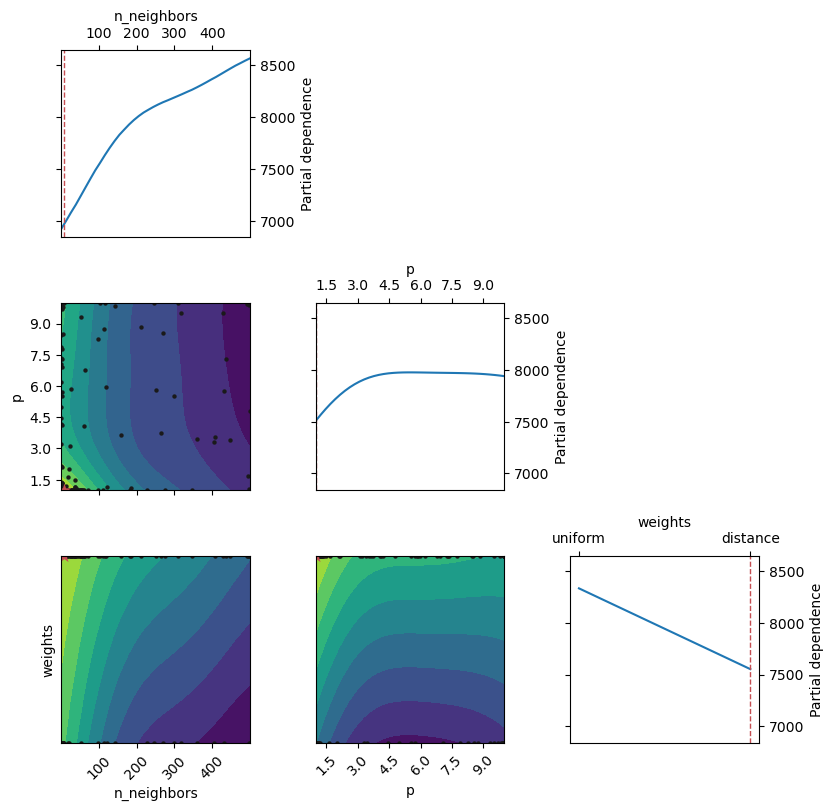

The frequence of individual hyperparameter values considered can also be visualized as below.

fig, ax = plt.subplots(1, 3, figsize = (10, 3))
plt.subplots_adjust(wspace=0.4)
plot_histogram(gcv.optimizer_results_[0], 0, ax = ax[0])
plot_histogram(gcv.optimizer_results_[0], 1, ax = ax[1])
plot_histogram(gcv.optimizer_results_[0], 2, ax = ax[2])
plt.show()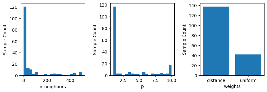

Below is the plot showing the minimum cross-validated score computed obtained until ‘n’ hyperparameter values are considered for cross-validation.

plot_convergence(gcv.optimizer_results_)
plt.show()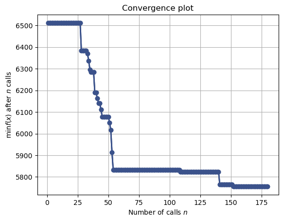

Note that the cross-validated error is close to the optmial value in the 53rd iteration itself.

The cross-validated error at the 53rd iteration is:

gcv.optimizer_results_[0]['func_vals'][53]

5831.87280274334

The hyperparameter values at the 53rd iterations are:

gcv.optimizer_results_[0]['x_iters'][53]

[15, 1.0, 'distance']

Note that this is the 2nd most optimal hyperparameter value based on GridSearchCV().

Below is the plot showing the cross-validated score computed at each of the 180 hyperparameter values considered for cross-validation. The plot shows that the algorithm seems to explore new regions of the domain space, instead of just exploting the promising ones. There is a balance between exploration and exploitation for finding the optimal hyperparameter values that minimize the objective function (i.e., the function that models the cross-validated score).

sns.lineplot(x = range(1, 181), y = gcv.optimizer_results_[0]['func_vals'])
plt.xlabel('Iteration')
plt.ylabel('Cross-validated score')
plt.show();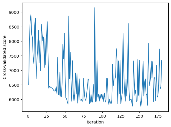

The advantages of BayesSearchCV() over GridSearchCV() and RandomizedSearchCV() are:

The Bayesian Optimization approach gives the benefit that we can give a much larger range of possible values, since over time we identify and exploit the most promising regions and discard the not so promising ones. Plain grid-search would burn computational resources to explore all regions of the domain space with the same granularity, even the not promising ones. Since we search much more effectively in Bayesian search, we can search over a larger domain space.
BayesSearch CV may help us identify the optimal hyperparameter value in fewer iterations if the Gaussian process model estimating the cross-validated score is relatively accurate. However, this is not certain. Grid and random search are completely uninformed by past evaluations, and as a result, often spend a significant amount of time evaluating “bad” hyperparameters.
BayesSearch CV is more reliable in cases of a large search space, where random selection may miss sampling values from optimal regions of the search space.

The disadvantages of BayesSearchCV() over GridSearchCV() and RandomizedSearchCV() are:

BayesSearchCV() has a cost of learning from past data, i.e., updating the model that predicts the cross-validated score after every iteration of evaluating the cross-validated score on a new hyperparameter value. This cost will continue to increase as more and more data is collected. There is no such cost in GridSearchCV() and RandomizedSearchCV() as there is no learning. This implies that each iteration of BayesSearchCV() will take a longer time than each iteration of GridSearchCV() / RandomizedSearchCV(). Thus, even if BayesSearchCV() finds the optimal hyperparameter value in fewer iterations, it may take more time than GridSearchCV() / RandomizedSearchCV() for the same.
The success of BayesSearchCV() depends on the predictions and associated uncertainty estimated by the Gaussian process (GP) model that predicts the cross-validated score. The GP model, although works well in general, may not be suitable for certain datasets, or may take a relatively large number of iterations to learn for certain datasets.

4.3.2 Live monitoring of cross-validated score

Note that it will be useful monitor the cross-validated score while the Bayesian Search CV code is running, and stop the code as soon as the desired accuracy is reached, or the optimal cross-validated score doesn’t seem to improve. The fit() method of the BayesSeaerchCV() object has a callback argument that can be used as follows:

model = KNeighborsRegressor(metric = 'minkowski') # No inputs defined inside the model
grid = {'n_neighbors': Integer(1, 500), 'weights': Categorical(['uniform', 'distance']), 
       'p': Real(1, 10, prior = 'uniform')} 

kfold = KFold(n_splits = 5, shuffle = True, random_state = 1)
gcv = BayesSearchCV(model, search_spaces = grid, cv = kfold, n_iter = 180, random_state = 10,
                         scoring = 'neg_root_mean_squared_error', n_jobs = -1)

paras = list(gcv.search_spaces.keys())
paras.sort()

def monitor(optim_result):
    cv_values = pd.Series(optim_result['func_vals']).cummin()
    display.clear_output(wait = True)
    min_ind = pd.Series(optim_result['func_vals']).argmin()
    print(paras, "=", optim_result['x_iters'][min_ind], pd.Series(optim_result['func_vals']).min())
    sns.lineplot(cv_values)
    plt.show()

gcv.fit(X_train_scaled, y_train, callback = monitor)

['n_neighbors', 'p', 'weights'] = [9, 1.0008321732366932, 'distance'] 5756.172382596493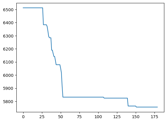

BayesSearchCV(cv=KFold(n_splits=5, random_state=1, shuffle=True),
              estimator=KNeighborsRegressor(), n_iter=180, n_jobs=-1,
              random_state=10, scoring='neg_root_mean_squared_error',
              search_spaces={'n_neighbors': Integer(low=1, high=500, prior='uniform', transform='normalize'),
                             'p': Real(low=1, high=10, prior='uniform', transform='normalize'),
                             'weights': Categorical(categories=('uniform', 'distance'), prior=None)})

4.4 `cross_validate()`

We have used cross_val_score() and cross_val_predict() so far.

When can we use one over the other?

The function cross_validate() is similar to cross_val_score() except that it has the option to return multiple cross-validated metrics, instead of a single one.

Consider the heart disease classification problem, where the response is target (whether the person has a heart disease or not).

data = pd.read_csv('Datasets/heart_disease_classification.csv')
data.head()

	age	sex	cp	trestbps	chol	fbs	restecg	thalach	exang	oldpeak	slope	thal	target
0	63	1	3	145	233	1	0	150	0	2.3	0	1	1
1	37	1	2	130	250	0	1	187	0	3.5	0	2	1
2	41	0	1	130	204	0	0	172	0	1.4	2	2	1
3	56	1	1	120	236	0	1	178	0	0.8	2	2	1
4	57	0	0	120	354	0	1	163	1	0.6	2	2	1

Let us pre-process the data.

# First, separate the response and the predictors
y = data['target']
X = data.drop('target', axis=1)

# Separate the data (X,y) into training and test

# Inputs:
    # data
    # train-test ratio
    # random_state for reproducible code
    
X_train, X_test, y_train, y_test = train_test_split(X, y, test_size=0.2, random_state=20, stratify=y) # 80%-20% split

# stratify=y makes sure the class 0 to class 1 ratio in the training and test sets are kept the same as the entire dataset.

model = KNeighborsClassifier() 
sc = StandardScaler()
sc.fit(X_train)
X_train_scaled = sc.transform(X_train)
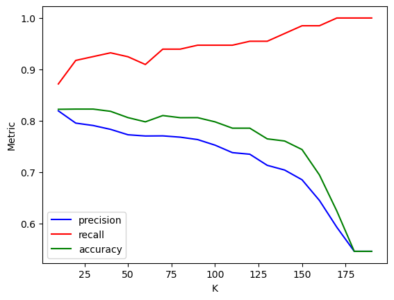
X_test_scaled = sc.transform(X_test)

Suppose we want to take recall above a certain threshold with the highest precision possible. cross_validate() computes the cross-validated score for multiple metrics - rest is the same as cross_val_score().

Ks = np.arange(10,200,10)

scores = []

for K in Ks:
    model = KNeighborsClassifier(n_neighbors=K) # Keeping distance uniform
    scores.append(cross_validate(model, X_train_scaled, y_train, cv=5, scoring = ['accuracy','recall', 'precision']))

scores

# The output is now a list of dicts - easy to convert to a df

df_scores = pd.DataFrame(scores) # We need to handle test_recall and test_precision cols

df_scores['CV_recall'] = df_scores['test_recall'].apply(np.mean)
df_scores['CV_precision'] = df_scores['test_precision'].apply(np.mean)
df_scores['CV_accuracy'] = df_scores['test_accuracy'].apply(np.mean)

df_scores.index = Ks # We can set K values as indices for convenience


#df_scores
# What happens as K increases?
    # Recall increases (not monotonically)
    # Precision decreases (not monotonically)
# Why?
    # Check the class distribution in the data - more obs with class 1
    # As K gets higher, the majority class overrules (visualized in the slides)
    # More 1s means less FNs - higher recall
    # More 1s means more FPs - lower precision
# Would this be the case for any dataset?
    # NO!! Depends on what the majority class is!

Suppose we wish to have the maximum possible precision for at least 95% recall.

The optimal ‘K’ will be:

df_scores.loc[df_scores['CV_recall'] > 0.95, 'CV_precision'].idxmax()

The cross-validated precision, recall and accuracy for the optimal ‘K’ are:

df_scores.loc[120, ['CV_recall', 'CV_precision', 'CV_accuracy']]

CV_recall       0.954701
CV_precision    0.734607
CV_accuracy     0.785374
Name: 120, dtype: object

sns.lineplot(x = df_scores.index, y = df_scores.CV_precision, color = 'blue', label = 'precision')
sns.lineplot(x = df_scores.index, y = df_scores.CV_recall, color = 'red', label = 'recall')
sns.lineplot(x = df_scores.index, y = df_scores.CV_accuracy, color = 'green', label = 'accuracy')
plt.ylabel('Metric')
plt.xlabel('K')
plt.show()

4.1 GridSearchCV

4.2 RandomizedSearchCV()

4.3 BayesSearchCV()